Background
Globally, there is an increasing demand for high quality beef that is flavorsome and tender, but also healthy and sustainably produced with high animal welfare standards. The same trend is observed in Korea, where consumers largely prefer the local Korean Hanwoo beef instead of imports, due to the juiciness, tenderness and high marbling levels of the breed (Hwang et al., 2010). In order to meet these consumer preferences, the key traits for meat quality are already included in the current selection index used by the national breeding program for the breed (Lee et al., 2014). More recently, genomic technologies, particularly genotyping marker panels of single nucleotide polymorphisms (SNP) have started to be more widely adopted by the industry which will, in time, lead to even higher rates of genetic gain.
Over the last ten years a broad range of SNP panels of varying densities have been commercialized in the form of SNP chips (arrays) and they have been used primarily for genomic selection applications. In cattle, there are low density panels that consist of only a few thousand SNP all the way up to the high-density panels with over a million markers; panel sizes between 50k and 150k are currently the most widely used as they provide a reasonable compromise between cost and number of markers. The number of SNP used is important for genomic selection since more markers increase the probability that at least one marker is in full or very high linkage disequilibrium (LD) with each genomic region involved in the genetic conformation of a trait of interest, even if the causal variant itself is not genotyped. The effects of all markers can then be estimated and the sum of these marker effects used to predict phenotype or breeding value.
More recently, whole-genome sequencing has become feasible in terms of costs and time; albeit still roughly 10 times more expensive than high-density commercial chips and it comes with a much higher computational overhead for the data analysis. The increase in prediction accuracy using sequence data in highly selected populations with small effective population sizes (e.g. Hanwoo) is marginal in comparison to high-density SNP arrays because of the high LD structure of these populations which is already well accounted for by lower density panels. It does, however, provide access to rare variants that are usually not present in commercial panels and, at least in principle, all causal variants should be in the sequence data. This is relevant since a significant proportion of the genetic variation may be due to rare alleles (Weller & Ron 2011) and there is no decay in linkage disequilibrium (van Binsbergen et al., 2014), which reduces the need to recalibrate prediction equations in the future.
Over the years, industry, breeding programs and research initiatives have invested heavily in the phenotyping and genotyping of large numbers of animals across the various SNP platforms. Since sequencing is still relatively expensive and to make the most of the historical data already collected; a widely used strategy is to sequence key representative animals from a population and then use this information to impute the sequence of the others. Imputation is a method to infer the unknown genotypes by exploring the information present in already known haplotypes. A wide range of programs have been developed to perform this task; for example Minimac3 (Howie et al., 2012), Beagle (Browning & Browning 2007), Impute2 (Howie et al., 2009), Fimpute (Sargolzaei et al., 2014), AlphaImpute (Hickey et al., 2012), Findhap (VanRaden et al., 2011), FastPhase (Scheet & Stephens 2006) and HSphase (Ferdosi et al., 2014). Each of these has its own strengths and weaknesses; some are faster, some are better for closely related populations, other work better with large unrelated populations; but overall no particular program is optimal across all scenarios. This makes it important to test different strategies and programs to identify the methodology best suited for the population of interest. Sometimes, programs can be combined to improve the accuracy of imputation, to reduce compute times that can be rather taxing or to find a balance between speed and accuracy. For example, in a comparison between Beagle and IMPUTE2, Brøndum et al., (2014) suggested that using BEAGLE for pre-phasing and IMPUTE2 for the imputation was a good strategy: better runtimes with only a marginal decrease in accuracy. Also, a study that evaluated the accuracy of sequence imputation in Fleckvieh and Holstein cattle (Pausch et al., 2017) noted that the combination of Eagle (Loh et al., 2016) and Minimac had a higher accuracy of imputation in comparison to Fimpute but this came at an increased computational cost and the need for a two-step approach; first a phasing step with Eagle followed by imputation with Minimac.
There are still few studies discussing sequence imputation but it is a very topic subject at the moment and the information needed to develop gold standards should emerge as new research is published in the near future. But for now, the broad steps for sequence imputation are to phase the haplotypes of the sequenced individuals and then use information from pedigree, family linkage and/or linkage disequilibrium to identify the combination of haplotypes for the animals with unknown markers (Huang et al., 2012). There are quite a few steps in this process to achieve an accurate sequence imputation within manageable runtimes. Herein, we describe, in practice, the steps needed to impute 50k SNP data up to sequence level with the help of a set of reference animals which were sequenced using the Illumina sequencing technology. A full script to run the imputation and an example dataset are available from the journal’s website as supplementary material:
(insert journal link).
>Materials
∙ 50k SNP genotypes from a number of individuals.
∙ SNP map. A file describing the genomic position of each marker.
∙ Reference sequence data and map from a number of individuals.
SNP data can come in various formats - a common one is the PLINK (Purcell et al., 2007) format. PLINK is a widely used and freely available software that implements several analyses for SNP data. Moreover, conveniently, commercially available SNP genotyping platforms can export directly to this format, including a genotype and an SNP map file.
To setup the imputation pipeline we will use PLINK v1.9 (Purcell et al., 2007), Eagle v2.3.5 (Loh et al., 2016), Minimac3 (Das et al., 2016). PLINK will be used to convert the data into a format suitable for use in Eagle and Minimac3. We will use Eagle to phase the data one chromosome at a time and Minimac3 will be used to impute the data up to sequence level guided by the reference sequences, also one chromosome at a time.
Methods
This section will guide you through the steps of the imputation process. Note that the example described herein is for Linux environments. We will use the statistical programming language R (R-Core-Team 2015) as a control center for the process. We will assume that all required software (PLINK, Eagle and Minimac3) are in the current working directory of R. The software is freely available and can be downloaded from:
PLINK: https://www.cog-genomics.org/plink/1.9/
Eagle: https://data.broadinstitute.org/alkesgroup/Eagle/
Minimac3: https://genome.sph.umich.edu/wiki/Minimac3
If the data is not in PLINK or vcf format but the data is available in GenomeStudio, it can be exported directly into PLINK from GenomeStudio. To do that you need to install the PLINK input report plug-in which can be downloaded from the following link: https://support.illumina.com/array/array_software/genomestudio/downloads.html, and then follow the steps described in the manual of the plug-in.
Imputation steps:
You will need the 50k data either in PLINK format or in vcf format, you also need the reference sequences in vcf format. The three main steps are as follows:
Step 1:If the 50k data is in PLINK binary or text format, you need to convert them into the vcf format, one chromosome at a time. This is because EAGLE will need the data in vcf format to phase them. For each chromosome, use EAGLE to phase the 50k vcf file.
Step 2:If you have whole reference sequence data as a single vcf file, split the data as a single chromosome vcf file using VCFtools (http://vcftools.sourceforge.net/) and phase them using EAGLE.
Step 3:Use Minimac3 to impute the 50k phased data using the phased reference data up to sequence level, one chromosome at a time.
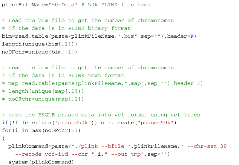
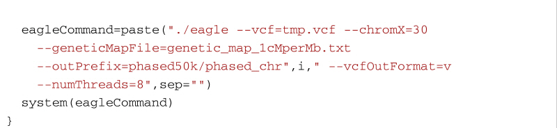
Step 1: Create vcf format files from PLINK binary or text file and phase them using Eagle
The code below will create a vcf file for each chromosome in the 50k dataset (27 files for the example in the supplementary material). You need the files 50kData.bed, 50kData.bim, and 50kData.fam in your working directory if the PLINK data is in binary format (supplementary material). Or, alternatively, 50kData.ped and 50kData.map if the data is in PLINK text format. For each chromosome PLINK will create an individual vcf file. Once PLINK creates a vcf format file for a chromosome, the code shown below then uses Eagle to phase it, and then the phased chromosome is stored in a folder named phased50k. If the folder does not exist in the working directory it will be automatically created when the code is executed for the first time. To phase the data, Eagles need a reference genetic map. If you are imputing cattle or sheep data use the map found in the file genetic_map_1cMperMb.txt that comes with the Eagle software (found in the tables folder of the software package). Put this file in the working directory. This is a generic map that is adequate for most purposes, but a user defined map with better information about distances can also be used. In a cluster environment, the number of CPUs can be set with the flag --numThreads. In the example below 8 CPUs are used.
An important point to consider when converting PLINK 1/2 allele format files into vcf files is that the PLINK ped and map files do not store information about the reference and alternate alleles in ACGT format. So, if the PLINK data is in ped and map formats and the alleles are coded as 1/2, the converted vcf file might not be compatible with other datasets (alleles may be flipped). When working with a genotype data file with 1/2 allele coding, it is necessary to determine whether the alleles are coded according to Illumina's A/B alleles or if they were simply recoded based on minor allele frequency using PLINK; if it's the latter, it is best to return the coding to the original genotype calls before doing anything further with the data.
To phase the example data with Eagle, open R, set the working directory to the folder with the data and use the code below:
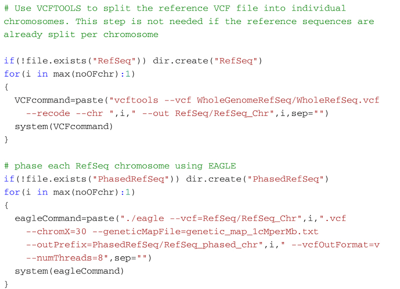
Step 2: Split the reference genome and phase one chromosome at a time using Eagle
If your reference genome sequence is in PLINK format then you can follow the same code from the previous section to split and phase the reference genomes. However, if the reference genomes are already in vcf format then, you will need to split the vcf file first, and then phase the output files using the Eagle software. To split the reference genome into individual chromosomes we can use VCFtools (http://vcftools.sourceforge.net/). The following code shows how to split the reference genome using VCFtools and then phase them using Eagle. It assumes that the whole reference genome sequence is stored in a folder WholeGenomeRefSeq and the VCFtools output will be stored in the folder RefSeq. Once the reference genomes have been split by VCFtools, the output files can be phased using Eagle as before. The phased reference genome will then be stored in the folder PhasedRefSeq.
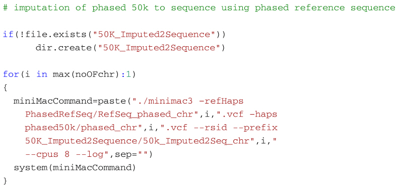
Step 3: Use Minimac3 to impute 50k phased data to sequence level
Once 50k and reference sequence data are phased, we can use Minimac3 to impute the 50k phased data up to sequence level. The imputed sequence data will be output into a directory 50K_Imputed2Sequence. By default, Minimac3 only accepts 1 - 22 as autosomes and this will cause errors when used to impute species with more than 22 autosomes (e.g. cattle or sheep data). To overcome this problem, a rather inelegant hack is to rename the chromosome field in the vcf files to a number between 1 - 22 for the autosomes beyond 22. But this process is rather inconvenient and a better approach is to modify and recompile the Minimac3 source code to accept up to e.g. 30 autosomes. Minimac3 is open source which makes it easy to make the change to accept a different number of autosomes. It is simply a matter of downloading the source files, then find the file src/HaplotypeSet.cpp in the distribution and open it using a text editor. Next find the function definition line bool HaplotypeSet::CheckValidChrom(string chr) at line 955 (in the current distribution) and replace lines 962-963 with the following code:
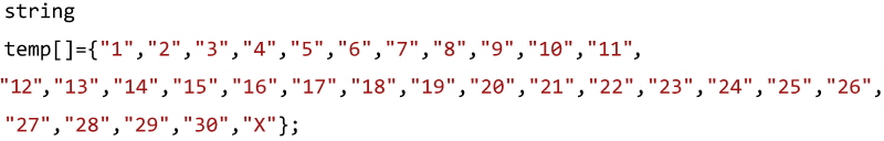
After this, save the file and recompile the program using the make command; now use this executable for the imputation:
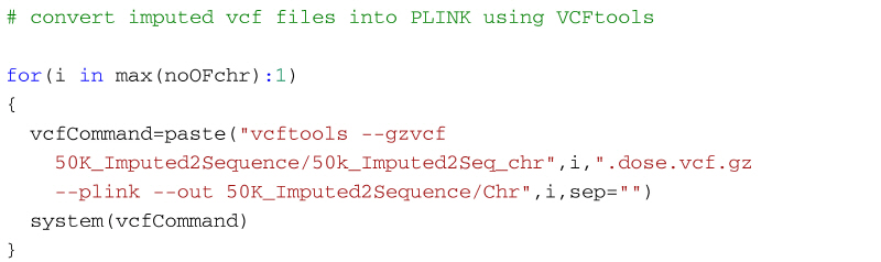
Once the imputation is complete we can create a PLINK format file or a genotype file from the imputed .vcf file using VCFtools. The following code will create the PLINK format file (ped and map files) from the imputed vcf file using VCFtools.
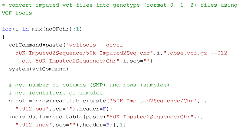
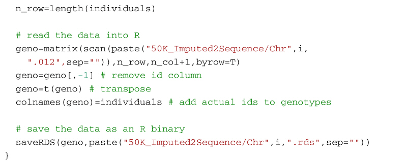
Alternatively, the following code will create a genotype file (format: 0, 1, 2) from the imputed vcf file using VCFtools for use in R. It first uses VCF tools to output the genotypes as a large matrix. It creates three files. The first, with suffix 012, contains the genotypes of each individual on a separate line. Genotypes are represented as 0, 1 and 2, where the number represents the number of non-reference alleles. Missing genotypes are represented by -1. The second file, with suffix 012.indv holds information of the individuals included in the main file; note that the identifiers (and genotypes) are reordered in relation to the original 50k data. The third file, with suffix 012.pos details the site locations (chromosome and location in base pairs) included in the main file. The SNP are ordered by base pair position but not all SNP from the 50k data will necessarily be in the final output, for example, for the dataset in the supplementary material, there are 13,140 SNP in the reference sequences but only 12,001 will be imputed in the final dataset. Some additional care is needed to match the output with the original SNP map file. The genotypes are then read into R using scan, and after some housekeeping, the matrix of genotypes is saved as an RDS file which is fast to read into R and not too demanding on disk space.

Quality control of imputed data
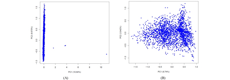
Once the imputation is complete, it is important to check the quality of the imputation and also the quality of the data before any further analysis. A full discussion about the QC of the imputed data is beyond the scope of this work; herein we will just briefly point out a couple of simple metrics that can be used. Minimac outputs a file with info extension that reports the quality of the imputation. Among the other columns, this info file has two columns named MAF (minor allele frequency) and Rsq (R2). We can filter the SNPs based on these two values. A ballpark figure is to discard those SNP that have Rsq<0.40 or MAF<0.01. Another quality control of the data is to plot the PCA of the genomic relationship matrix (GRM) to check if there are any samples with poor imputation. Figure 1 shows two PCA plots where Figure 1 (a) has a few bad samples and Figure 1 (b) shows the same PCA plot after removing these bad samples. The latter can be illustrated with the following code:
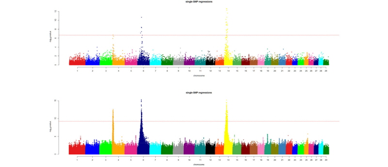
After quality control of the imputed data, we are ready for downstream analysis. Common uses of the imputed data are GWAS and genomic prediction. Imputation greatly improves the resolution of the GWAS results. Figure 2 shows a comparison of GWAS results for 24 months body weight of Korean Hanwoo cattle using 2,100 animals with 50k data and imputed data (~15 million SNP). The QTL peaks are better resolved and other putative regions, even if not significant in a statistical sense, are more separable from the background noise.
Conclusion
In this tutorial, we described the main steps for imputation of low density (50k) SNP data up to sequence level using a sequenced reference dataset. The same process can be used to impute data from 50k to 700k or from 700k to sequence level. For the phasing and imputation steps we used two freely available programs (Eagle and Minimac); out of the current pool of software available for phasing and imputation, these two perform very well. This simple roadmap can be used, in practice, for phasing and imputation of livestock genomic datasets, adding additional value to the large numbers of animals already genotyped on the various platforms.