Transcriptome profiling
Information representing biological phenomena is encoded in the genome. Therefore, it is possible to identify the genes of each living organism through genome analysis and infer their characteristics and similarities to each other. Not all genes in the genome are always expressed, but living organisms respond to the external environment by expressing their genes according to specific circumstances. Transcriptome analysis is used for determining how an organism responds by comparing and confirming the expression level of a gene (Wolf, 2013).
1. Representative transcriptome profiling methods
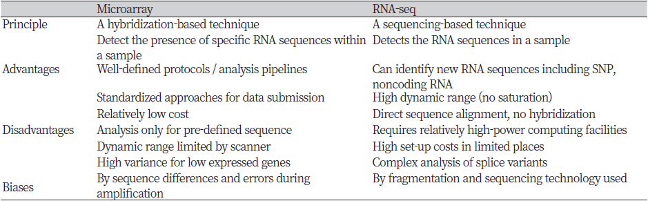
The most popular genome-wide transcriptome profiling methods are to use microarray and RNA-sequencing (RNA-seq) (Table 1). Microarray is based on the hybridization of target strands with fixed complementary probe strands which are consisted of already known sequences. RNA derived from characteristic cells is treated with reverse transcriptase to make complementary DNA (cDNA), and then a fluorescent substance is added thereon to examine the level of gene expression (Ekins & Chu, 1999). Microarray has the advantage of confirming the result through a relatively simple reaction, and chips for specific organisms are commercially available. Since the microarray technique has been developed and commercialized a long time ago, its standards are well established and reliability is also high. On the other hand, the RNA-seq method is based on next-generation sequencing (NGS) that reads all RNA sequences. It converts cDNA from each isolated transcript and then sequencing them with a massively parallel deep sequencing-based approach. The resulting short sequencing reads can be mapped to a reference genome to quantify the expression level of a gene relative to a condition of interest or absolute level (Wang, Gerstein, & Snyder, 2009). In the past, the microarray technique played an important role in whole transcriptome analysis. However, nowadays, RNA-seq has been preferred because it effectively overcomes the limitations of microarray. RNA-seq technology is not dependent on the prior knowledge of the reference transcriptome, unlike the microarray. Also, when compared to microarray, RNA-seq data includes a higher dynamic range of expression levels, lower background signals, and a relatively small amount of total RNA for quantification (Van Vliet, 2010).
2. Other transcriptome profiling methods
Serial analysis of gene expression (SAGE) is a sequence-based approach transcriptome technology that can be identified and quantitatively compared. It generates a short specific tag of a population of messenger RNA (mRNA) in a sample of interest based on generating a representative SAGE tags library. SAGE sequencing allows the high-throughput process of the frequency of libraries correlating with the relative amounts of their mRNAs (Velculescu, Zhang, Vogelstein, & Kinzler, 1995). In addition, massively parallel signature sequencing (MPSS) is the sequencing tool that is available to conduct in-depth expression profiling. It is an open-ended platform that counts the number of individual mRNA molecules produced by each gene and can be analyzed at the expression level. The datasets of MPSS are in a simplified digital format and no prior requirements are needed to identify and characterize the genes (Rani & Sharma, 2017; Reinartz et al., 2002).
Atlas
Over the decades, scientists have strived to provide a comprehensive overview of research findings in the field of genomics. As a result, a growing number of overviews for different types of research have been published, and one of the most effective research methods that contain the entire content was constructing a biological atlas. The purpose of a biological atlas is to assist users by providing additional information and analyses of maps. In particular, the structure of the human body, including the location of bones and muscles, and nerves, is the most often shown in anatomy (Netter, 2014). There are also many atlases containing comprehensive genetic information, and it is possible to check the contents and use the database online.
1. Types of atlas
A brief introduction to representative atlas databases made for easy use by people: (1) The human protein atlas which is composed of 6 detailed atlas (tissue atlas, single cell type atlas, pathology atlas, brain atlas, blood atlas, and cell atlas) (Pontén, Jirström, Uhlen, & Ireland, 2008). The aim of this atlas is to map all human proteins by integrating system biology techniques such as antibody-based imaging and mass spectrometry-based proteomics. (2) The cancer genome atlas (TCGA) contains comprehensive information including molecular characteristics of the major cancer genome of over 20,000 primary cancer and matched normal samples spanning 33 cancer types (Weinstein et al., 2013). (3) The Allen brain atlas is a genome-wide atlas that integrates gene expression information and anatomical data generated in the mouse brain. In addition, the brain atlas maps and identifies genes expressed in all tissues of the brain in a three-dimensional space (Sunkin et al., 2012).
2. Methodologies of genomic atlas
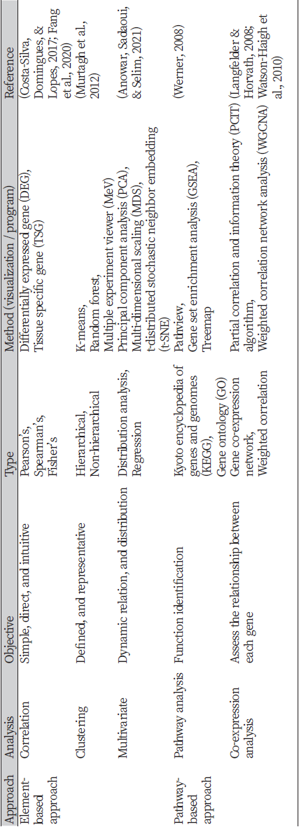
There are several ways to display genomic information, and some of the main methods used in the transcriptome atlas are as follows (Table 2). Firstly, analyses such as multi-dimensional scaling (MDS), t-distributed stochastic neighbor embedding (t-SNE), and principal component analysis (PCA) are performed to check the similarity and distribution pattern of the data (Abdi & Williams, 2010; Hout, Papesh, & Goldinger, 2013; Van der Maaten & Hinton, 2008). Similarly, hierarchical clustering analysis is used to categorize samples with similar characteristics. There are various types of cluster agglomeration methods such as maximum or complete linkage clustering, minimum or single linkage clustering, mean or average linkage clustering, centroid linkage clustering, and Ward’s minimum variance method, and the linkage method is selected differently among Euclidean distance, Manhattan distance, Pearson correlation distance, Spearman correlation distance, and Kendall correlation distance according to the characteristics of the data (Murtagh, Contreras, & Discovery, 2012). Through genetic location mapping, specific locations where genes are expressed can be identified by mapping genes or genetic variants to the expressed tissue or further to the expressed chromosome (Altshuler, Daly, & Lander, 2008; Mahfouz, Huisman, Lelieveldt, Reinders, & Function, 2017). In addition, this approach allows for annotating the reference genome to identify already known genomes and their biological function using a genome browser and other functional annotation databases. Furthermore, gene co-expression network (GCN) analysis is performed to find the correlation between genes and significant biomarkers among the genes inside the network. Representative examples of this analysis are using the partial correlation and information theory (PCIT) algorithm (Watson-Haigh, Kadarmideen, & Reverter, 2010) and the weighted gene co-expression network analysis (WGCNA) (Langfelder & Horvath, 2008). The selected biomarker can be subjected to subsequent analysis, such as showing changes in expression level or analyzing their function compared to other species (Fang et al., 2020).
Endocrine disrupting chemicals (EDCs)
1. Types of EDC
Endocrine disrupting chemicals (EDCs), which are also known as environmental hormones, are chemicals that cause various diseases by disrupting the normal function of the endocrine system in the body. It is largely divided into naturally occurring EDC and synthetic EDC (Kabir, Rahman, Rahman, & pharmacology, 2015). Heavy metals such as lead, cadmium, and mercury are known as naturally occurring EDC. The first known synthetic EDC was diethylstilbestrol (DES), a powerful synthetic female hormone. It was administered to millions of pregnant women in the United States from 1948 to 1972, with the hope that it would be effective in preventing miscarriage, while the efficacy and safety of the drug had not been confirmed in clinical trials. Unfortunately, miscarriages increased, and the fetus would have a disorder of the reproductive system (Langston, 2008). Phytoestrogens, which exist in nature as endocrine disruptors, have been observed to have estrogen activity in more than 43 edible plants such as bean, apple, cherry, strawberry, wheat, corn, and cotton fruit. It is known that the concentration of these hormones is known to be only about a few thousandths of the natural estrogen secreted by the body, so in general, these foods do not act as endocrine disruptors (Reinli, Block, & cancer, 1996). The category of endocrine disruptors that has been the most problematic in recent years is environmental pollutants. Since they are both endocrine disruptors and environmental pollutants, they are sometimes referred to as environmental endocrine disruptors. Currently, more than 100 species are known. Typical examples are bisphenol analogs, dioxin, polychlorinated biphenyls (PCBs), dichloro-diphenyl-trichloroethane (DDT), organic chlorine pesticides, heavy metals, and plasticizers (Diamanti-Kandarakis et al., 2009).
2. Bisphenol A
Bisphenol A (BPA), an endocrine disrupting chemical that permeates daily life from receipts to plastic bags, is threatening human health (Rochester, 2013). In the case of infants and children, due to behavioral characteristics such as sucking fingers or sitting on the floor, the concentration of endocrine disruptors accumulated in the body is high, so caution is required. In particular, it was confirmed that the concentration of BPA in the urine of infants and children was twice that of adults. A typical problem with BPA exposure in children and adolescents is precocious puberty. In addition, BPA is a substance capable of binding to androgen receptors and inhibits spermatogenesis by antagonizing androgens at high concentrations (Radwan et al., 2018). BPA is an endocrine disruptor that has been proven to be the most correlated with obesity, and according to the US National Health and Nutrition Examination Survey, higher BPA concentration in both adults and children are associated with a higher risk of obesity and abdominal obesity (Carwile & Michels, 2011). An association between BPA and cardiovascular disease was reported in the 2008 US National Health and Nutrition Examination Survey data analysis (Lang et al., 2008). Similarly, a 10-year follow-up in the UK also showed that an increase in BPA concentration of 4.56 ng/ml increased the risk of coronary artery disease by 1.13 times, suggesting a correlation between BPA and cardiovascular disease (Melzer et al., 2012).