
Seung-Wan Woo  1 , Jaemin Kim 1,2 , Woncheoul Park 3,*
1Division of Applied Life Science (BK21), Gyeongsang National University, Jinju 52828, Republic of Korea
2Institute of Agriculture and Life Sciences, Gyeongsang National University, Jinju 52828, Republic of Korea
3Animal Genetics & Breeding Division, National Institute of Animal Science, Rural Development Administration, Cheonan 31000, Republic of Korea
*Corresponding author: wcpark1982@korea.kr
Volume 10, Number 3, Pages 133–148, September 2026.
Journal of Animal Breeding and Genomics 2026, 10(3), 133–148. https://doi.org/10.12972/jabng.2026.10.3.4
Received on August 31, 2026, Revised on September 28, 2026, Accepted on September 28, 2026, Published on September 30, 2026.
Copyright © 2026 Korean Society of Animal Breeding and Genetics.
This is an Open Access article distributed under the terms of the Creative Commons Attribution Non-Commercial License (https://creativecommons.org/licenses/by-nc/4.0/) which permits unrestricted non-commercial use, distribution, and reproduction in any medium, provided the original work is properly cited.

16S rRNA gene, Hanwoo, microbiome, QIIME 2
The digestive tract microbiome contributes to host nutrient digestion and absorption, metabolism, and immune homeostasis, among other physiological processes (Round and Mazmanian, 2009; Sekirov et al., 2010; Rowland et al., 2018). Its composition and function vary along the gastrointestinal tract with local differences in the host environment (Donaldson et al., 2016). In ruminants, the stomach is divided into four compartments: the rumen, reticulum, omasum, and abomasum. These compartments differ in physicochemical conditions such as pH, oxygen concentration, and digesta retention time, and each one harbors a distinct microbial community (Tardiolo et al., 2025). The compartment-specific microbial communities are associated with digestive efficiency and systemic metabolism (Xue et al., 2020). Amplicon sequencing of the hypervariable regions of the 16S rRNA gene is a widely used standard method for analyzing microbial communities in a culture-independent manner (Caporaso et al., 2011; Klindworth et al., 2013). The raw sequence data are processed through a series of bioinformatic steps before taxonomic composition and microbial diversity can be compared across samples. QIIME 2 is a widely used platform that integrates these processing steps into one pipeline (Bolyen et al., 2019).
Hanwoo is an economically important Korean native beef breed, and research has been conducted on a variety of traits in this breed (Bedhane et al., 2019; Haque et al., 2024; Jang et al., 2024). In Hanwoo steers, the rumen microbiota has been associated with marbling score (Kim et al., 2020). Rumen alpha diversity has also been correlated with carcass traits (Kang et al., 2024). Feed efficiency has been associated with the fecal microbiota (Park et al., 2026). Relating the microbiota of different gastrointestinal sites to these traits involves sampling several sites from each animal. Comparisons between sites within the same animal require statistical tests that account for the pairing between samples.
Several general workflows are available for 16S rRNA amplicon analysis, such as the Bioconductor workflow and Microbiome Helper, but they are not specific to paired designs (Callahan et al., 2016b; Comeau et al., 2017). Statistical approaches for paired samples have been described separately, including random effects in ANCOM-BC2 and MaAsLin2, and restricted permutations in vegan (Mallick et al., 2021; Lin and Peddada, 2024; Oksanen et al., 2026). This protocol describes a step-by-step workflow for comparing the microbial communities of the rumen (RUM) and abomasum (ABO) using 16S rRNA amplicon sequencing data from Hanwoo steers. It covers primer and adapter trimming, DADA2-based denoising and amplicon sequence variant (ASV) inference, SILVA-based taxonomic classification, phylogenetic tree construction, alpha and beta diversity comparison, relative abundance profiling, and differential abundance testing between RUM and ABO with ANCOM-BC2 and MaAsLin2 (Figure 1). It aims to provide a reproducible workflow for comparing microbial community composition and diversity between RUM and ABO samples from the same animals, accounting for the pairing in the statistical analyses.
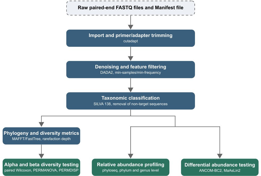
Figure 1. Overview of the analysis workflow. Steps performed in QIIME 2 are shown in blue, and steps performed in R are shown in green. PERMANOVA: permutational multivariate analysis of variance; PERMDISP: permutational analysis of multivariate dispersions.
The 16S rRNA amplicon sequencing data supporting this protocol are available from the NCBI SRA database (BioProject PRJNA1452526). The dataset provides paired-end reads for 124 samples, one rumen (RUM) and one abomasum (ABO) sample from each of 62 Hanwoo steers. The reads were generated by amplifying the V3–V4 region of the 16S rRNA gene with the 341F (5′-CCTACGGGNGGCWGCAG-3′) and 805R (5′-GACTACHVGGGTATCTAATCC-3′) primer pair on an Illumina MiSeq platform. Sequence processing was performed in QIIME 2 (v2023.9), and downstream statistical analyses were performed in R (v4.2.2) using the packages summarized in Table 1. The tools, input files, output files, and key parameters of each step are summarized in Table 2. The QIIME 2 environment was created using conda (v22.9.0) and the environment file for the QIIME 2 amplicon distribution.
Table 1. Software tools used in this protocol
| Software tool | Version | Purpose |
|---|---|---|
| QIIME 2 | v2023.9 | Primer trimming, denoising, taxonomic classification, phylogeny, diversity analysis |
| R | v4.2.2 | Statistical analysis |
| qiime2R | v0.99.6 | Import QIIME 2 artifacts directly into R |
| phyloseq | v1.42.0 | Taxonomic aggregation, relative abundance calculation |
| vegan | v2.7-3 | PERMANOVA, PERMDISP |
| ANCOMBC (ANCOM-BC2) | v2.0.2 | Differential abundance testing |
| MaAsLin2 | v1.12.0 | Differential abundance testing |
| PERMANOVA: permutational multivariate analysis of variance; PERMDISP: permutational analysis of multivariate dispersions. | ||
Table 2. Summary of the analysis steps, tools, input files, output files, and key parameters
| Step | Tool/plugin | Input | Output | Key parameters |
|---|---|---|---|---|
| Import | QIIME 2 | FASTQ files, manifest file | Dataset.qza | –input-format |
| Primer and adapter trimming | q2-cutadapt | Dataset.qza | Dataset_trimmed.qza | –p-front-f, –p-front-r, –p-adapter-f, –p-adapter-r |
| Denoising | q2-dada2 | Dataset_trimmed.qza | Dataset_table.qza, Dataset_repseqs.qza | –p-trunc-len-f, –p-trunc-len-r |
| Feature filtering, taxonomic classification, and non-target removal | q2-feature-table, q2-feature-classifier, q2-taxa | Dataset_table.qza, Dataset_repseqs.qza | Dataset_repseqs_noneu. qza, Dataset_table_noneu.qza | –p-min-samples, –p-min-frequency, –p-exclude |
| Phylogeny and diversity metrics | q2-phylogeny, q2- diversity | Dataset_repseqs_noneu.qza, Dataset_table_noneu.qza | Rooted_tree.qza, Core-metrics-results | –p-sampling-depth |
| Alpha and beta diversity testing | R (vegan) | Exported diversity.tsv files, Manifest file | Test statistics and p-values | wilcox.test, adonis2, betadisper |
| Relative abundance profiling | R (qiime2R, phyloseq) | Dataset_table_noneu.qza, Dataset_taxonomy.qza | Dataset_table_assigned. qza, Relative abundance | taxrank |
| Differential abundance | R (ANCOMBC, MaAsLin2) | Dataset_table_assigned.qza, Dataset_taxonomy.qza | Effect size, standard error, p-value, q-value | fix_formula, rand_formula, prv_cut, fixed_effects, random_effects, min_prevalence |
conda env create \
--name qiime2-amplicon-2023.9 \
--file https://raw.githubusercontent.com/qiime2/distributions/refs/heads/dev/2023.9/amplicon/released/qiime2-amplicon-ubuntu-latest-
conda.yml
conda activate qiime2-amplicon-2023.9The raw data consist of paired-end FASTQ files, in which each read is represented by four lines containing the read identifier, nucleotide sequence, separator line, and per-base quality scores. QIIME 2 does not analyze FASTQ files directly, so the reads are first imported into a QIIME 2 artifact (.qza), a zip archive containing the data together with metadata describing its type and provenance. Each QIIME 2 action takes artifacts as input and produces artifacts or visualizations as output. Visualization files (.qzv) can be opened with QIIME 2 View (https:// view.qiime2.org). The data inside an artifact can be exported to standard formats such as .tsv with the qiime tools export command.
Paired-end FASTQ files for all 124 libraries were imported into QIIME 2 as ʻSampleData[PairedEndSequencesWithQuality]’ using the qiime tools import command. The import used a manifest in ʻPairedEndFastqManifestPhred33V2’, which lists the absolute paths of the forward and reverse FASTQ files for each library. The manifest is a tab-separated text file with one row per library and contains the columns ʻsample-id’, ʻforward-absolute-filepath’, and ʻreverse-absolute-filepath’, followed by the tissue and animal identifier columns. The tissue and animal identifier columns were subsequently used as sample metadata in downstream analyses.
qiime tools import \
--type 'SampleData[PairedEndSequencesWithQuality]' \
--input-path Manifest_file \
--input-format PairedEndFastqManifestPhred33V2 \
--output-path Dataset.qzaThe q2-cutadapt plugin identifies and removes primer and adapter sequences from sequencing reads by local alignment (Martin, 2011). Primers were removed with the ʻtrim-paired’ action in two sequential steps. The first step trimmed the 341F and 805R primers from the 5′ end with ʻ–p-front-f’ and ʻ–p-front-r’ and discarded reads with no detected primer through ʻ–p-discard-untrimmed’.
qiime cutadapt trim-paired \
--i-demultiplexed-sequences Dataset.qza \
--p-front-f CCTACGGGNGGCWGCAG \
--p-front-r GACTACHVGGGTATCTAATCC \
--p-discard-untrimmed \
--o-trimmed-sequences Dataset_trimmed_front.qza
The second step trimmed the reverse complement of the opposite primer from the 3′ end with ʻ–p-adapter-f’ and ʻ–p-adapter-r’ and kept reads in which no adapter was detected. Two steps were needed because one 5′ primer-trimming pass does not remove the 3′ adapter that is read through when an amplicon is shorter than the sequencing read. Reads were discarded at the 5′ step so that only reads with an intact primer continued, and reads were kept at the 3′ step because most V3–V4 amplicons are longer than the read and do not reach the opposite primer. The two trimming steps retained 11,734,675 of 11,922,261 raw read pairs (98.43%).
qiime cutadapt trim-paired \
--i-demultiplexed-sequences Dataset_trimmed_front.qza \
--p-adapter-f GGATTAGATACCCBDGTAGTC \
--p-adapter-r CTGCWGCCNCCCGTAGG \
--o-trimmed-sequences Dataset_trimmed.qza
qiime demux summarize \
--i-data Dataset_trimmed.qza \
--o-visualization Dataset_trimmed.qzv
The sequence quality summary of the trimmed reads shows the per-base quality-score distributions used to determine the truncation lengths in the next step (Figure 2). Median forward-read quality remained near a Phred quality score of 38 up to position 220, then gradually decreased toward position 280. Reverse-read quality began decreasing earlier, from around position 180, with the decline becoming more pronounced beyond position 220.
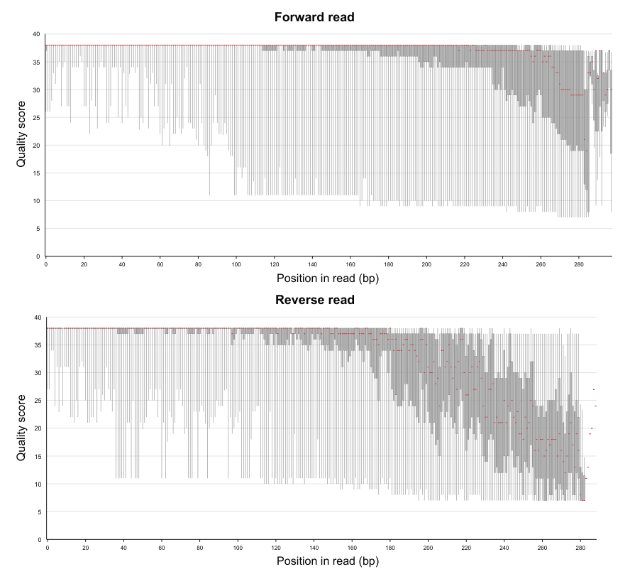
Figure 2. Per-base quality score distribution for forward and reverse reads after primer and adapter trimming. Red marks indicate the median quality score at each position. These distributions were used to select DADA2 truncation lengths.
The q2-dada2 plugin denoises the reads with an error model learned from the data, infers exact ASVs, merges the forward and reverse reads, and removes chimeras (Callahan et al., 2016a). Denoising was performed with the ʻdenoise-paired’ action. The forward and reverse reads were truncated to 280 bp and 220 bp with ʻ–p-trunc-len-f’ and ʻ–p-trunc-len-r’, respectively. No bases were trimmed from the read starts because the primers had already been removed, and chimeras were removed with the consensus method. The reverse reads were truncated at 220 bp because the decline in quality became more pronounced beyond this position (Figure 2). The resulting ASVs were 285–466 bp long (median 420 bp) after primer removal. The combined truncated length of 500 bp left a forward-reverse overlap of 34–215 bp (median 80 bp), calculated as 500 bp minus the length of each ASV sequence. Even the shortest overlap was well above the default minimum of 12 bp for merging. Of the denoised read pairs, 83.62% were merged (per-sample median 82.61%, range 57.98–97.99%). DADA2 retained 5,914,998 non-chimeric read pairs, which was 50.41% of the trimmed read pairs and 49.61% of the raw read pairs. Per-sample retention of the raw read pairs had a median of 48.71% (range 22.08–77.86%). This step produces a feature table, the representative sequences, and per-sample denoising statistics. The read pairs remaining after each step are shown in Table 3. Truncation lengths depend on the primer set and the read length, so the values used and the resulting overlap should be reported.
Table 3. Read pairs and ASVs retained at each processing step
| Step | Read pairs (n) | Percentage of raw read pairs (%) | ASVs (n) |
|---|---|---|---|
| Raw read pairs | 11,922,261 | 100.00 | – |
| After cutadapt step 1 (5′ primer) | 11,736,785 | 98.44 | – |
| After cutadapt step 2 (3′ adapter) | 11,734,675 | 98.43 | – |
| DADA2 quality filtering | 8,599,358 | 72.13 | – |
| DADA2 denoising | 7,609,246 | 63.82 | – |
| DADA2 merging | 6,363,111 | 53.37 | – |
| After chimera removal | 5,914,998 | 49.61 | 28,566 |
| After feature filtering (min-samples 2, min-frequency 10) | 5,688,064 | 47.71 | 8,944 |
| After removing mitochondria, chloroplast, and Eukaryota | 5,686,996 | 47.70 | 8,927 |
| After removing Unassigned | 5,686,996 | 47.70 | 8,927 |
| ASV: amplicon sequence variant. |
qiime dada2 denoise-paired \
--i-demultiplexed-seqs Dataset_trimmed.qza \
--p-trim-left-f 0 \
--p-trunc-len-f 280 \
--p-trim-left-r 0 \
--p-trunc-len-r 220 \
--p-chimera-method consensus \
--o-representative-sequences Dataset_repseqs.qza \
--o-table Dataset_table.qza \
--o-denoising-stats Dataset_stats.qzaThe q2-feature-table plugin provides operations to filter, summarize, and transform the ASV table. Features were filtered with the ʻfilter-features’ action in two steps. Features present in fewer than two samples were removed with ʻ–p-min-samples 2’, and the result was filtered with ʻ–p-min-frequency 10’ to remove features with a total frequency below 10. Representative sequences were then matched to the filtered table with ʻfilter-seqs’ to retain the same ASV set across both files. Features detected in only a single sample are more likely to reflect contamination or sequencing artifacts, and features with very low total frequency are difficult to estimate reliably across samples. Both thresholds were set low to limit the loss of rare taxa, and the total-frequency cutoff should be considered relative to library depth.
qiime feature-table filter-features \
--i-table Dataset_table.qza \
--p-min-samples 2 \
--o-filtered-table Dataset_table_filtering.qza
qiime feature-table filter-features \
--i-table Dataset_table_filtering.qza \
--p-min-frequency 10 \
--o-filtered-table Dataset_table_frequency_filtering.qza
qiime feature-table filter-seqs \
--i-data Dataset_repseqs.qza \
--i-table Dataset_table_frequency_filtering.qza \
--o-filtered-data Dataset_repseqs_filtering.qzaThe q2-feature-classifier plugin trains and applies taxonomic classifiers for marker-gene reads. A naive Bayes classifier assigns each representative sequence to the most probable taxonomy based on its k-mer composition, using a labeled reference dataset for training (Bokulich et al., 2018). The V3–V4 region was extracted in silico from the SILVA release 138 SSURef NR99 reference sequences with ʻextract-reads’ using the 341F and 805R primers (Quast et al., 2013). The reference files ʻsilva-138-99-seqs.qza’ and ʻsilva-138-99-tax.qza’ were obtained from the QIIME 2 2023.9 data resources (https://docs.qiime2.org/2023.9/data-resources/). A naive Bayes classifier was trained on the extracted region with ʻfit-classifier-naive-bayes’ and applied with ʻclassify-sklearn’ at the default confidence of 0.7. All other parameters were left at the default values.
qiime feature-classifier extract-reads \
--i-sequences silva-138-99-seqs.qza \
--p-f-primer CCTACGGGNGGCWGCAG \
--p-r-primer GACTACHVGGGTATCTAATCC \
--o-reads silva_138_99_341F_805R.qza
qiime feature-classifier fit-classifier-naive-bayes \
--i-reference-reads silva_138_99_341F_805R.qza \
--i-reference-taxonomy silva-138-99-tax.qza \
--o-classifier silva_138_99_341F_805R_classifier.qza
qiime feature-classifier classify-sklearn \
--i-classifier silva_138_99_341F_805R_classifier.qza \
--i-reads Dataset_repseqs_filtering.qza \
--o-classification Dataset_taxonomy.qza
ASVs assigned to mitochondria, chloroplasts, or eukaryotes were then removed from the table and the representative sequences with ʻtaxafilter-table’, ʻtaxa filter-seqs’, and the ʻ–p-exclude’ option.
qiime taxa filter-table \
--i-table Dataset_table_frequency_filtering.qza \
--i-taxonomy Dataset_taxonomy.qza \
--p-exclude mitochondria,chloroplast,Eukaryota \
--o-filtered-table Dataset_table_noneu.qza
qiime taxa filter-seqs \
--i-sequences Dataset_repseqs_filtering.qza \
--i-taxonomy Dataset_taxonomy.qza \
--p-exclude mitochondria,chloroplast,Eukaryota \
--o-filtered-sequences Dataset_repseqs_noneu.qza
Training on the amplified region rather than on full-length 16S rRNA gene sequences improves genus-level accuracy for short reads, because the reference k-mer profiles then match the length and coverage of the query reads (Werner et al., 2012). Mitochondrial, chloroplast, and eukaryotic sequences were removed because the 341F and 805R primers also amplify host mitochondrial and dietary chloroplast 16S rRNA. These non-target sequences inflate diversity estimates and distort relative abundance.
The ʻqiime phylogeny align-to-tree-mafft-fasttree’ pipeline aligns the representative sequences using MAFFT, masks highly gapped or poorly conserved alignment columns, constructs an approximately maximum-likelihood tree using FastTree, and midpoint-roots the resulting tree (Price et al., 2010; Katoh and Standley, 2013). The ʻqiime diversity core-metrics-phylogenetic’ pipeline rarefies the table to a fixed depth and then computes alpha and beta diversity metrics from the rarefied table and the rooted phylogenetic tree in a single step.
qiime phylogeny align-to-tree-mafft-fasttree \
--i-sequences Dataset_repseqs_noneu.qza \
--o-alignment aligned_repseqs.qza \
--o-masked-alignment masked_aligned_repseqs.qza \
--o-tree unrooted_tree.qza \
--o-rooted-tree rooted_tree.qza
qiime diversity core-metrics-phylogenetic \
--i-phylogeny rooted_tree.qza \
--i-table Dataset_table_noneu.qza \
--p-sampling-depth 8300 \
--m-metadata-file Manifest_file \
--output-dir core-metrics-results
qiime tools export \
--input-path core-metrics-results/Diversity.qza \
--output-path core-metrics-results/Diversity_for_R
The ʻalign-to-tree-mafft-fasttree’ pipeline was run with default parameters. The ʻcore-metrics-phylogenetic’ pipeline was also run with default parameters except for the rarefaction depth. This depth specifies the number of reads to which each sample is subsampled, and samples with fewer reads than this depth are excluded. The rarefaction depth was set to 8,300 reads, corresponding to the minimum per-sample read count in the filtered feature table, so that all samples were retained. Only one library had fewer than 10,000 reads, and a depth of 8,300 reads was 17.5% of the median library size (47,390.5 reads). A depth of 10,000 reads would have excluded this library and its paired sample, resulting in the exclusion of one individual from the paired analysis. This step produces alpha diversity metrics (Shannon entropy, Faith’s phylogenetic diversity, Pielou’s evenness, observed ASVs) and beta diversity distance matrices (Bray-Curtis, Jaccard, weighted UniFrac, unweighted UniFrac). These outputs were exported as .tsv files for downstream analysis in R.
RUM and ABO samples were collected from the same 62 individuals. The two samples from each animal share between-animal variation and therefore cannot be considered independent observations. Alpha diversity metrics were compared using paired Wilcoxon signed-rank tests, with the individual as the experimental unit, rather than using a test that assumes two independent groups. Ignoring the pairing treats between- animal variation as noise and may reduce statistical power to detect differences between tissues. The same rationale applies to the permutational multivariate analysis of variance (PERMANOVA) and differential abundance analyses described below. For each alpha diversity metric, the exported values were merged with the sample metadata and restructured, with each individual contributing one row containing paired RUM and ABO values. The test was conducted separately for each of the four metrics. The results were then combined, and the p-values were adjusted across the four tests using the Benjamini–Hochberg method.
library(dplyr)
library(tidyr)
metric_col <- "alpha_diversity"
df <- read.table(Alpha_file, header = FALSE, skip = 1, stringsAsFactors = FALSE)
colnames(df) <- c("SampleID", metric_col)
meta <- read.table(Manifest_file, header = TRUE, sep = "\t",
stringsAsFactors = FALSE, check.names = FALSE)
meta_clean <- meta %>%
select(SampleID = `sample-id`, Animal = Sample, Group = Tissue) %>%
mutate(Group = toupper(trimws(Group)))
df_joined <- df %>%
left_join(meta_clean, by = "SampleID")
df_wide <- df_joined %>%
select(Animal, Group, all_of(metric_col)) %>%
pivot_wider(names_from = Group, values_from = all_of(metric_col))
wt <- wilcox.test(df_wide$RUM, df_wide$ABO, paired = TRUE)
write.table(data.frame(metric = metric_col, p_value = wt$p.value),
paste0(metric_col, "_wilcoxon.tsv"), sep = "\t", row.names = FALSE, quote = FALSE)
# Run once per metric, then combine and BH-adjust
alpha_files <- list.files(pattern = "_wilcoxon\\.tsv$")
alpha_stats <- do.call(rbind, lapply(alpha_files, read.delim))
alpha_stats$q_value <- p.adjust(alpha_stats$p_value, method = "BH")
PERMANOVA tests whether community composition differs between groups by partitioning variation in a distance matrix among sources of variation and comparing the observed test statistic with a permutation-based null distribution. Permutational analysis of multivariate dispersions (PERMDISP) tests whether multivariate dispersion differs between groups. Because the two samples from the same animal are not independent, permutations were restricted so that tissue labels were shuffled only within each animal. Each animal contributed one RUM and one ABO sample, so in each permutation, its two tissue labels were either retained or swapped, thereby preserving the pairing. For each of the four beta-diversity metrics, distances were compared between RUM and ABO samples with tissue as the grouping variable, using the ʻadonis2’ and ʻbetadisper’ functions from the vegan package with 9,999 permutations (Oksanen et al., 2026). The animal identifier was specified as the ʻstrata’ argument in ʻadonis2’, and the sample metadata were reordered to match the distance matrix. PERMDISP was performed because a significant PERMANOVA result can arise from unequal dispersion rather than differences in group centroids. For PERMDISP, the residuals of the distances to the group centroids were permuted within each animal in the same manner, using the ʻblocks’ argument of the ʻhow’ function. For each metric, the PERMANOVA R2, PERMANOVA p-value, and PERMDISP p-value were written to the summary file. The R2 represents the proportion of variation in community composition explained by tissue.
library(vegan)
metric_label <- "beta_diversity"
dist_matrix_raw <- read.table(Beta_file, header = TRUE, sep = "\t",
check.names = FALSE)
rownames(dist_matrix_raw) <- dist_matrix_raw[[1]]
dist_matrix <- as.dist(as.matrix(dist_matrix_raw[, -1]))
meta <- read.table(Manifest_file, header = TRUE, sep = "\t",
stringsAsFactors = FALSE, check.names = FALSE)
meta_aligned <- meta[match(labels(dist_matrix), meta$`sample-id`), ]
permanova_fit <- adonis2(dist_matrix ~ Tissue, data = meta_aligned,
permutations = 9999, strata = meta_aligned$Sample)
permanova_p <- permanova_fit[1, "Pr(>F)"]
permanova_r2 <- permanova_fit[1, "R2"]
dispersion_fit <- betadisper(dist_matrix, meta_aligned$Tissue)
permdisp_p <- permutest(dispersion_fit, permutations = how(nperm = 9999,
blocks = meta_aligned$Sample))$tab[1, "Pr(>F)"]
beta_stats_row <- data.frame(metric = metric_label, n_samples = nrow(meta_aligned),
permanova_p = permanova_p, permanova_r2 = permanova_r2, permdisp_p = permdisp_p)
write.table(beta_stats_row, "beta_diversity_stats.tsv", sep = "\t",
row.names = FALSE, quote = FALSE)The qiime2R package imports QIIME 2 artifacts directly into R, and phyloseq stores the feature table, taxonomy, sample metadata, and tree in a single object and provides functions for taxonomic agglomeration and abundance transformation (McMurdie and Holmes, 2013; Bisanz, 2018). This step requires every retained feature to have a taxonomic assignment. A feature without a taxonomic assignment cannot be placed in a taxon and would form a single mixed category in the relative abundance profiles and the differential abundance analyses. Features without a taxonomic assignment were removed using ʻtaxa filter-table’ and ʻ–p-exclude Unassigned’. No features were removed at this step because all ASVs remaining after removal of mitochondrial, chloroplast, and eukaryotic sequences had received a taxonomic assignment at the classifier confidence threshold of 0.7. Features assigned only at a higher taxonomic rank were not removed and were retained as unclassified at lower ranks. Relative abundances were calculated for each sample after this step.
qiime taxa filter-table \
--i-table Dataset_table_noneu.qza \
--i-taxonomy Dataset_taxonomy.qza \
--p-exclude Unassigned \
--o-filtered-table Dataset_table_assigned.qza
The table, taxonomy, and metadata were read into a phyloseq object (qza_to_phyloseq). ASVs were summed within each taxon at a specified rank (tax_glom), and taxa were retained (prune_taxa) if they were detected in at least a set fraction of samples. Relative abundances were then calculated for each sample (transform_sample_counts) and averaged within each tissue. ASVs were agglomerated at the phylum and genus levels. At each rank, a taxon was kept only if it occurred in at least 10% of the 124 combined RUM and ABO samples. The 10% prevalence cutoff was applied to show taxa present across the dataset rather than taxa driven by one or two samples. The prevalence fraction should be reported, because it is a user-defined threshold that affects reproducibility.
library(qiime2R)
library(phyloseq)
library(dplyr)
library(tidyr)
library(tibble)
table_qza <- "Dataset_table_assigned.qza"
taxonomy_qza <- "Dataset_taxonomy.qza"
meta_file <- "Manifest_file"
physeq <- qza_to_phyloseq(features = table_qza, taxonomy = taxonomy_qza,
metadata = meta_file)
rank <- "taxa_rank" # Phylum or Genus
glom <- tax_glom(physeq, taxrank = rank, NArm = FALSE)
tax_df <- as.data.frame(as.matrix(tax_table(glom)))
taxa_names(glom) <- make.unique(as.character(tax_df[[rank]]))
otu <- otu_table(glom)
if (!taxa_are_rows(glom)) otu <- t(otu)
min_samples <- ceiling(nsamples(glom) * 0.1)
keep <- rowSums(otu > 0) >= min_samples
glom <- prune_taxa(keep, glom)
relative_abundance <- transform_sample_counts(glom, function(x) if (sum(x) == 0) x
else x / sum(x))
ra_long <- as.data.frame(t(as(otu_table(relative_abundance), "matrix"))) %>%
rownames_to_column("SampleID") %>%
pivot_longer(cols = -SampleID, names_to = "Taxon", values_to = "RA") %>%
left_join(data.frame(sample_data(relative_abundance)) %>%
rownames_to_column("SampleID") %>%
select(SampleID, Tissue), by = "SampleID")
mean_ra <- ra_long %>%
group_by(Tissue, Taxon) %>%
summarise(MeanAbundance = mean(RA), .groups = "drop")ANCOM-BC2 models the observed counts using a linear model on a log scale after estimating and correcting for sample-specific samplingfractions and taxon-specific sequencing efficiencies, and reports a bias-corrected log fold change for each taxon with its standard error (Lin and Peddada, 2024). MaAsLin2 fits a taxon-specific linear model to normalized and transformed abundances and reports a coefficient for each covariate (Mallick et al., 2021). The MaAsLin2 model can be extended to a linear mixed-effects model when random effects are specified. Both methods were performed at the phylum and genus levels with tissue as the fixed effect and individual identity as a random effect. RUM was used as the reference tissue, a 10% prevalence filter was applied to the dataset, and the Benjamini–Hochberg method was used to adjust p-values, with q-value < 0.05 considered significant. For ANCOM-BC2, all samples were retained regardless of the library size (lib_cut = 0). Taxa absent or nearly absent in one tissue were classified as structural zeros rather than tested directly (struc_zero = TRUE), using the asymptotic lower bound to detect structural zeros (neg_lb = TRUE). For MaAsLin2, sample abundances were scaled by total sum scaling (TSS) and log-transformed (normalization = “TSS”, transform = “LOG”), and a linear mixed-effects model was fitted rather than a count- based model (analysis_method = “LM”). The normalization, transformation, and analysis method used here correspond to the default settings of MaAsLin2. Mallick et al. (2021) reported that TSS showed the best balance of performance among the normalization methods tested, and that linear models were the only class of methods that controlled the false discovery rate across study designs, with moderate power. Because ANCOM-BC2 does not have a reference argument, the reference level of the tissue factor was set before model fitting. MaAsLin2 instead takes the reference through its ʻreference’ argument.
library(ANCOMBC)
sample_data(glom)$Tissue <- factor(sample_data(glom)$Tissue,
levels = c("RUM", "ABO"))
ancombc2(data = glom,
fix_formula = "Tissue", rand_formula = "(1 | Sample)", group = "Tissue",
struc_zero = TRUE, neg_lb = TRUE, prv_cut = 0.1, lib_cut = 0,
p_adj_method = "BH", alpha = 0.05)
library(Maaslin2)
feature_table <- as(otu_table(glom), "matrix")
if (taxa_are_rows(glom)) feature_table <- t(feature_table)
feature_table <- as.data.frame(feature_table)
metadata <- data.frame(sample_data(glom))
Maaslin2(input_data = feature_table, input_metadata = metadata,output = paste0("maaslin2_", rank), fixed_effects = "Tissue",
random_effects = "Sample", reference = "Tissue,RUM", normalization = "TSS",
transform = "LOG", analysis_method = "LM", correction = "BH",
min_prevalence = 0.1, max_significance = 0.05)Under this parameterization, a positive value indicates enrichment in ABO and a negative value indicates enrichment in RUM. The direction of the effect depends on which tissue is the reference. The same reference was used for both methods to ensure comparability of results. Because differential abundance tools can yield inconsistent results even with the same data, two independent methods were applied (Nearing et al., 2022). The results from each method are visualized as bar plots (Figure 3).
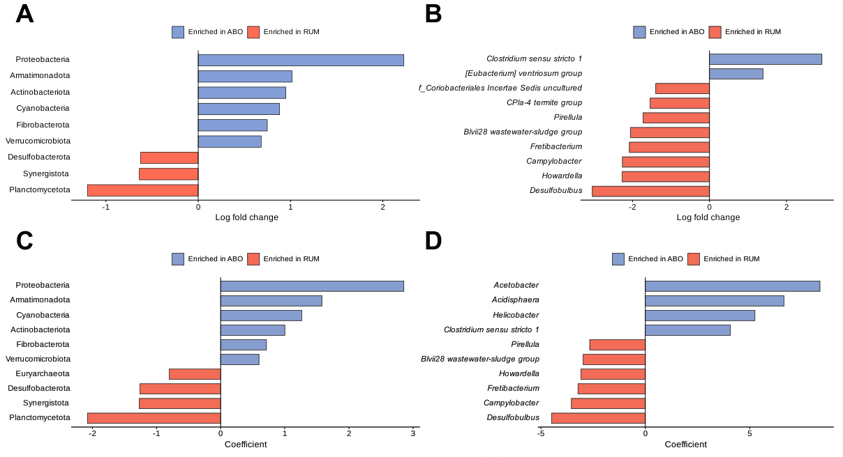
Figure 3. Differentially abundant taxa between RUM and ABO. (A) Phylum-level taxa identified by ANCOM-BC2. (B) Genus-level taxa identified by ANCOM-BC2. (C) Phylum-level taxa identified by MaAsLin2. (D) Genus-level taxa identified by MaAsLin2. ANCOM-BC2 results are shown as log fold change, and MaAsLin2 results are shown as the coefficient. Up to the top 10 taxa by effect size are shown in each panel, colored by the tissue in which each taxon was enriched. RUM: rumen; ABO: abomasum.
This protocol describes a reproducible workflow for comparing the microbial communities of the rumen and abomasum using publicly available 16S rRNA amplicon sequencing data from Hanwoo steers. Primer and adapter trimming, DADA2 denoising, SILVA-based classification, alpha and beta diversity comparison, relative abundance profiling, and differential abundance testing using ANCOM-BC2 and MaAsLin2 were performed, with paired statistical designs used for comparisons between RUM and ABO samples. The workflow can be adapted to other paired microbiome comparisons, such as other gastric compartments or matched tissue sites, and potentially to other animal species. However, parameter settings should be evaluated for each new dataset. Primer sequences, truncation lengths, filtering thresholds, rarefaction depth, and prevalence cutoffs depend on the dataset and should be reviewed before applying the workflow to new data.
None.
Conceptualization: Woo SW, Kim J, Park W. Data curation: Woo SW, Park W. Formal analysis: Woo SW. Methodology: Woo SW, Kim J. Software: Woo SW. Visualization: Woo SW. Resources: Park W. Writing – original draft: Woo SW. Writing – review & editing: Kim J, Park W. Supervision: Kim J, Park W. Project administration: Park W. Funding acquisition: Park W. All authors read and approved the final manuscript.
No potential conflict of interest relevant to this article is reported.
Animal protocols were approved by the Institutional Animal Care and Use Committee of the National Institute of Animal Science (NIAS),Rural Development Administration, Republic of Korea (approval no. NIAS20201979).
This study was supported by a grant from the Cooperative Research Program for Agriculture Science & Technology Development (Project no. PJ01492004), RDA, Republic of Korea.
During the preparation of this work, the authors used generative AI to improve the language quality and grammar of this manuscript. The authors reviewed and edited the content as needed and take full responsibility for the content of this publication.
Bedhane M, van der Werf J, Gondro C, et al. 2019. Genome-wide association study of meat quality traits in Hanwoo beef cattle using imputed whole-genome sequence data. Frontiers in Genetics 10:1235. https://doi.org/10.3389/fgene.2019.01235
Bisanz JE. 2018. qiime2R: Importing QIIME2 artifacts and associated data into R sessions. R package version 0.99.6. https://github.com/jbisanz/ qiime2R (Accessed August 30, 2026).
Bokulich NA, Kaehler BD, Rideout JR, et al. 2018. Optimizing taxonomic classification of marker-gene amplicon sequences with QIIME 2's q2- feature-classifier plugin. Microbiome 6:90. https://doi.org/10.1186/s40168-018-0470-z
Bolyen E, Rideout JR, Dillon MR, et al. 2019. Reproducible, interactive, scalable and extensible microbiome data science using QIIME 2. Nature Biotechnology 37:852–857. https://doi.org/10.1038/s41587-019-0209-9
Callahan BJ, McMurdie PJ, Rosen MJ, et al. 2016a. DADA2: High-resolution sample inference from Illumina amplicon data. Nature Methods 13:581–583. https://doi.org/10.1038/nmeth.3869
Callahan BJ, Sankaran K, Fukuyama JA, et al. 2016b. Bioconductor workflow for microbiome data analysis: From raw reads to community analyses. F1000Research 5:1492. https://doi.org/10.12688/f1000research.8986.2
Caporaso JG, Lauber CL, Walters WA, et al. 2011. Global patterns of 16S rRNA diversity at a depth of millions of sequences per sample. Proceedings of the National Academy of Sciences of the United States of America 108(Suppl 1):4516–4522. https://doi.org/10.1073/ pnas.1000080107
Comeau AM, Douglas GM, Langille MGI. 2017. Microbiome Helper: A custom and streamlined workflow for microbiome research. mSystems 2(1):e00127-16. https://doi.org/10.1128/mSystems.00127-16
Donaldson GP, Lee SM, Mazmanian SK. 2016. Gut biogeography of the bacterial microbiota. Nature Reviews Microbiology 14:20–32. https:// doi.org/10.1038/nrmicro3552
Haque MA, Lee YM, Ha JJ, et al. 2024. Genome-wide association study identifies genomic regions associated with key reproductive traits in Korean Hanwoo cows. BMC Genomics 25:496. https://doi.org/10.1186/s12864-024-10401-3
Jang S, Jang S, Kim J, et al. 2024. Multi-tissue transcriptome analysis to identify candidate genes associated with weight regulation in Hanwoo cattle. Frontiers in Genetics 14:1304638. https://doi.org/10.3389/fgene.2023.1304638
Kang R, Song J, Park JK, et al. 2024. Impact of forage sources on ruminal bacteriome and carcass traits in Hanwoo steers during the late fattening stages. Microorganisms 12(10):2082. https://doi.org/10.3390/microorganisms12102082
Katoh K, Standley DM. 2013. MAFFT multiple sequence alignment software version 7: Improvements in performance and usability. Molecular Biology and Evolution 30(4):772–780. https://doi.org/10.1093/molbev/mst010
Kim M, Park T, Jeong JY, et al. 2020. Association between rumen microbiota and marbling score in Korean native beef cattle. Animals 10(4):712. https://doi.org/10.3390/ani10040712
Klindworth A, Pruesse E, Schweer T, et al. 2013. Evaluation of general 16S ribosomal RNA gene PCR primers for classical and next-generation sequencing-based diversity studies. Nucleic Acids Research 41(1):e1. https://doi.org/10.1093/nar/gks808
Lin H, Peddada SD. 2024. Multigroup analysis of compositions of microbiomes with covariate adjustments and repeated measures. Nature Methods 21:83–91. https://doi.org/10.1038/s41592-023-02092-7
Mallick H, Rahnavard A, McIver LJ, et al. 2021. Multivariable association discovery in population-scale meta-omics studies. PLoS Computational Biology 17(11):e1009442. https://doi.org/10.1371/journal.pcbi.1009442
Martin M. 2011. Cutadapt removes adapter sequences from high-throughput sequencing reads. EMBnet.journal 17(1):10–12. https:// doi.org/10.14806/ej.17.1.200
McMurdie PJ, Holmes S. 2013. phyloseq: An R package for reproducible interactive analysis and graphics of microbiome census data. PLoS ONE 8(4):e61217. https://doi.org/10.1371/journal.pone.0061217
Nearing JT, Douglas GM, Hayes MG, et al. 2022. Microbiome differential abundance methods produce different results across 38 datasets. Nature Communications 13:342. https://doi.org/10.1038/s41467-022-28034-z
Oksanen J, Simpson GL, Blanchet FG, et al. 2026. vegan: Community ecology package. R package version 2.7-3. https://cran.r-project.org/ package=vegan (Accessed August 30, 2026). https://doi.org/10.32614/CRAN.package.vegan
Park C, Kim MS, Yu Z, et al. 2026. Effect of divergent residual feed intake on the fecal microbiota in fattening Hanwoo steers. Scientific Reports 16:8075. https://doi.org/10.1038/s41598-026-39485-5
Price MN, Dehal PS, Arkin AP. 2010. FastTree 2 – Approximately maximum-likelihood trees for large alignments. PLoS ONE 5(3):e9490. https:// doi.org/10.1371/journal.pone.0009490
Quast C, Pruesse E, Yilmaz P, et al. 2013. The SILVA ribosomal RNA gene database project: Improved data processing and web-based tools. Nucleic Acids Research 41(D1):D590–D596. https://doi.org/10.1093/nar/gks1219
Round JL, Mazmanian SK. 2009. The gut microbiota shapes intestinal immune responses during health and disease. Nature Reviews Immunology 9:313–323. https://doi.org/10.1038/nri2515
Rowland I, Gibson G, Heinken A, et al. 2018. Gut microbiota functions: Metabolism of nutrients and other food components. European Journal of Nutrition 57:1–24. https://doi.org/10.1007/s00394-017-1445-8
Sekirov I, Russell SL, Antunes LCM, et al. 2010. Gut microbiota in health and disease. Physiological Reviews 90:859–904. https://doi.org/10.1152/ physrev.00045.2009
Tardiolo G, La Fauci D, Riggio V, et al. 2025. Gut microbiota of ruminants and monogastric livestock: An overview. Animals 15(5):758. https:// doi.org/10.3390/ani15050758
Werner JJ, Koren O, Hugenholtz P, et al. 2012. Impact of training sets on classification of high-throughput bacterial 16s rRNA gene surveys. The ISME Journal 6:94–103. https://doi.org/10.1038/ismej.2011.82
Xue MY, Sun HZ, Wu XH, et al. 2020. Multi-omics reveals that the rumen microbiome and its metabolome together with the host metabolome contribute to individualized dairy cow performance. Microbiome 8:64. https://doi.org/10.1186/s40168-020-00819-8