
Dahyun Park  1 , Haesu Ko 2 , Tae-Sung Hwang 3 , Jaemin Kim 1,4,*
1Division of Applied Life Science (BK21), Gyeongsang National University, Jinju 52828, Republic of Korea
2Animal Genomics and Bioinformatics Division, National Institute of Animal Science, Rural Development Administration, Wanju 55365, Republic of
Korea
3Institute of Animal Medicine, College of Veterinary Medicine, Gyeongsang National University, Jinju 52828, Republic of Korea
4Institute of Agriculture and Life Sciences, Gyeongsang National University, Jinju 52828, Republic of Korea
*Corresponding author: jmkim85@gnu.ac.kr
Volume 10, Number 3, Pages 119–132, September 2026.
Journal of Animal Breeding and Genomics 2026, 10(3), 119–132. https://doi.org/10.12972/jabng.2026.10.3.3
Received on August 31, 2026, Revised on September 21, 2026, Accepted on September 22, 2026, Published on September 30, 2026.
Copyright © 2026 Korean Society of Animal Breeding and Genetics.
This is an Open Access article distributed under the terms of the Creative Commons Attribution Non-Commercial License (https://creativecommons.org/licenses/by-nc/4.0/) which permits unrestricted non-commercial use, distribution, and reproduction in any medium, provided the original work is properly cited.

consensus clustering, gene expression, median absolute deviation, transcriptomics, unsupervised clustering
Gene expression profiles provide quantitative information that can be used to examine molecular variation among biological samples. Even samples within the same phenotypic or experimental group may exhibit heterogeneous expression patterns, and identifying this heterogeneity can reveal previously unrecognized molecular subgroups. Unsupervised clustering is therefore widely used to explore expression datasets without requiring predefined class labels (Guinney et al., 2015). The results of unsupervised clustering, however, can be influenced by the genes included in the analysis, differences in expression scale, clustering parameters, and the number of clusters specified. Feature selection is particularly important for high-dimensional expression datasets, since genes showing little variation across samples provide limited information for distinguishing sample groups. Median absolute deviation (MAD) provides a simple and robust measure of expression variability and can be used to prioritize highly variable genes for subsequent clustering. Standardization of the selected genes, such as gene-wise Z-score transformation, further enables comparison of expression patterns across genes with different expression ranges. In addition to appropriate feature selection and standardization, the stability of the identified sample groups should also be considered. Consensus clustering assesses this stability by repeatedly clustering resampled subsets of the data and measuring how consistently pairs of samples are assigned to the same cluster. ConsensusClusterPlus provides several outputs for evaluating candidate cluster solutions, including consensus matrices, cumulative distribution function (CDF) curves, and cluster consensus scores. Additional measures, such as the proportion of ambiguous clustering (PAC), can be used to quantify uncertainty in sample grouping.
Selecting the final number of clusters is not always straightforward, since different measures of clustering stability may favor different values of K, so candidate solutions are best evaluated using multiple complementary measures rather than a single criterion. In this technical protocol, we describe a step-by-step workflow that takes a processed logCPM expression matrix as its starting point and proceeds through MAD-based feature selection, gene-wise Z-score transformation, consensus clustering, and evaluation of candidate cluster numbers. A processed logCPM expression dataset containing 11 case samples is used as an example to demonstrate implementation of the workflow (Figure 1).
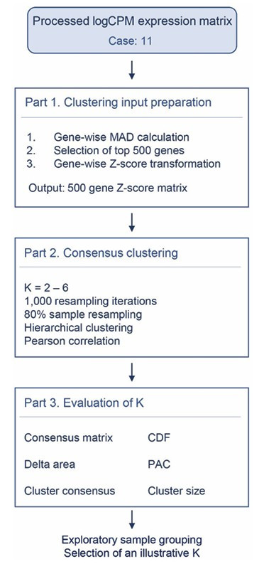
Figure 1. Overview of the exploratory consensus clustering workflow for gene expression data. CDF: cumulative distribution function; K: number of clusters; logCPM: log-transformed counts per million; MAD: median absolute deviation; PAC: proportion of ambiguous clustering.
The workflow requires a tab-delimited processed gene expression matrix in which rows represent genes and columns represent individual samples. The first column should contain unique gene identifiers, while each subsequent column should correspond to an individual sample and contain numeric expression values. The example provided in Supplementary Table 1 contains logCPM values. Missing or non-numeric values should be removed or resolved before analysis. Genes with zero variance across samples should be excluded before Z-score transformation.
For the worked example, a processed and de-identified logCPM expression matrix comprising 11 case samples was used solely to demonstrate the computational workflow. The example dataset is presented at the processed expression-matrix level because the purpose of this Technical Protocol is to demonstrate the implementation and evaluation of the consensus clustering workflow using processed gene expression data. The processed matrix required to reproduce the workflow from the feature-selection step is provided in Supplementary Table 1. Briefly, raw count data were filtered using filterByExpr and normalized using calcNormFactors in edgeR, followed by voom transformation in limma. The resulting processed logCPM matrix was used as the example input for subsequent feature selection and consensus clustering (Liu et al., 2014). The software tools and computational environments used in the workflow are summarized in Table 1.
Table 1. Software tools and computational environments used for consensus clustering
| Category | Software | Version | Application |
|---|---|---|---|
| Expression data processing | edgeR | v3.38.4 | Filtering and normalization |
| Expression data processing | limma | v3.52.4 | logCPM transformation |
| Input data preparation | Python | v2.7.5 | MAD calculation and Z-score transformation |
| Consensus clustering | ConsensusClusterPlus | v1.62.0 | Consensus clustering and cluster stability assessment |
| Statistical analysis | R | v4.5.0 | Statistical analysis and visualization |
| Visualization | ggplot2 | v4.0.3 | Visualization of clustering results |
| logCPM: log-transformed counts per million; MAD: median absolute deviation. | |||
Highly variable genes were selected from the provided logCPM matrix before consensus clustering. Genes showing little variation across samples provide limited information for distinguishing expression patterns among samples. Therefore, genes with relatively high variability were selected before clustering.
Gene variability was evaluated using median absolute deviation (MAD) (Howell, 2005). For each gene, the median expression value across samples was calculated, and the absolute deviation of each expression value from the median was then computed. The median of these absolute deviations was used as the MAD value. Higher MAD values indicate greater expression variability across samples. MAD values were calculated in Python using the provided logCPM expression matrix. Genes were ranked by MAD, and the 500 genes with the highest MAD values were selected for subsequent analysis. The top 500 genes were selected as a practical feature set size for demonstrating the workflow, rather than as a biologically optimized or universally applicable threshold. Because the number of selected features can influence clustering results, sensitivity to feature-set size was additionally assessed by repeating the consensus clustering analysis using the top 1,000 and 1,500 MAD-ranked genes. This step reduced the expression matrix to a subset of genes showing the greatest variation across samples.
Before consensus clustering, the expression values of the selected genes were standardized using gene-wise Z-score transformation. For each gene, the mean expression value across samples was subtracted from each expression value and divided by the standard deviation of that gene. This transformation placed genes with different expression ranges on a comparable scale while preserving their relative expression patterns across samples. The resulting matrix contained Z-score-transformed expression values for the 500 selected genes, with genes arranged in rows and samples in columns. The matrix was saved as a tab-delimited text file and used as the input for consensus clustering (Figure 2).
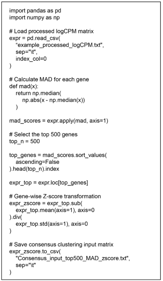
Figure 2. Python code for preparing the expression matrix ahead of consensus clustering. The code shows the sequential steps of gene variability calculation using median absolute deviation (MAD), selection of the 500 genes with the highest MAD values, and gene-wise Z-score transformation to generate the input matrix for consensus clustering. logCPM: log-transformed counts per million; MAD: median absolute deviation.
Consensus clustering was performed using the ConsensusClusterPlus package in R (Wilkerson and Hayes, 2010; Şenbabaoğlu et al., 2014). The Z-score-transformed matrix containing the 500 genes selected according to MAD was imported into R and converted to a numeric matrix (Ihaka and Gentleman, 1996). Genes were maintained in rows and samples in columns. The purpose of consensus clustering was to determine whether samples could be reproducibly separated into groups based on similarities in their overall expression patterns rather than on predefined sample labels.
Unlike a single application of a clustering algorithm, consensus clustering repeatedly performs clustering on resampled subsets of the data. The results from these repeated analyses are then combined to assess how consistently individual samples are grouped. Sample pairs that repeatedly occur in the same cluster across resampling iterations provide evidence for a stable grouping, whereas pairs whose assignments frequently change indicate greater clustering uncertainty. Candidate cluster numbers from K = 2 to K = 6 were evaluated by setting maxK = 6. Thus, five candidate clustering solutions were examined. For each candidate K, the clustering procedure was repeated 1,000 times (reps = 1,000). Repeated resampling was used to evaluate whether the observed grouping of samples remained consistent when the clustering procedure was performed using different subsets of the dataset.
In each iteration, 80% of the samples were randomly selected by setting pItem = 0.8. Consequently, individual clustering iterations were performed on partially overlapping subsets rather than the complete sample set. This procedure allows cluster stability to be evaluated according to whether samples continue to be grouped together when the composition of the analyzed subset changes. All 500 selected genes were retained in every iteration (pFeature = 1), meaning that resampling was applied to samples but not to genes.
Hierarchical clustering was specified as the clustering algorithm (clusterAlg = "hc"). Similarity among samples was evaluated using Pearson correlation (distance = "pearson"). Hierarchical clustering was performed using average linkage for both the inner clustering step and the final consensus clustering step (innerLinkage = "average" and finalLinkage = "average"), consistent with the default settings of ConsensusClusterPlus. Pearson correlation emphasizes similarity in the expression patterns across the selected genes rather than similarity based solely on the absolute magnitudes of individual expression values. This is particularly appropriate after gene-wise Z-score transformation because clustering is intended to identify samples exhibiting similar relative expression profiles across the selected features (Goder and Filkov, 2008).
A random seed of 1234 was specified before clustering to ensure reproducibility of the resampling procedure. Using the same input matrix, software settings, and random seed therefore allows the same sequence of resampling operations and cluster evaluation to be reproduced. The main clustering parameters are summarized in Table 2.
Table 2. Main parameters used for consensus clustering with ConsensusClusterPlus
| Parameter | Example setting | Description |
|---|---|---|
| maxK | 6 | Maximum number of clusters evaluated |
| reps | 1,000 | Number of resampling iterations |
| pItem | 0.8 | Proportion of samples included in each iteration |
| pFeature | 1.0 | Proportion of genes included in each iteration |
| clusterAlg | hc | Hierarchical clustering |
| distance | Pearson | Distance based on Pearson correlation |
| innerLinkage | average | Linkage method used for inner clustering |
| finalLinkage | average | Linkage method used for final consensus clustering |
| seed | 1234 | Random seed used for reproducibility |
| K: number of clusters; maxK: maximum number of clusters; reps: number of resampling iterations; pItem: proportion | ||
| of items (samples) sampled per iteration; pFeature: proportion of features (genes) sampled per iteration; hc: hierarchical | ||
| clustering. | ||
For each candidate K, the results of the 1,000 clustering iterations were summarized as a consensus matrix. The consensus value for a pair of samples represents the proportion of eligible resampling iterations in which those two samples were assigned to the same cluster. Consensus values range from 0 to 1. A value approaching 1 indicates that the two samples were consistently grouped together whenever both were included in the resampled dataset, whereas a value approaching 0 indicates that they were consistently assigned to different clusters (Figure 3).
The consensus matrix, therefore, provides a direct representation of clustering stability at the sample-pair level. A well-defined cluster is expected to contain samples with high within-cluster consensus values, while consensus values between samples assigned to different clusters should remain low. In contrast, intermediate consensus values indicate that sample relationships are less consistently reproduced across resampling iterations.
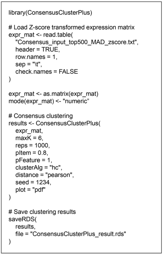
Figure 3. R workflow for consensus clustering using ConsensusClusterPlus. The code shows consensus clustering of the Z-score-transformed expression matrix for K = 2 to K = 6. Clustering was repeated 1,000 times using 80% of the samples and all 500 selected genes in each iteration, with hierarchical clustering and Pearson correlation. K: number of clusters; logCPM: log-transformed counts per million.
Consensus matrices were generated for each candidate solution from K = 2 through K = 6. Cumulative distribution function (CDF) plots were also generated to summarize the distribution of consensus values at each K. The complete ConsensusClusterPlus output was saved as an RDS file so that the same clustering results could subsequently be used to calculate and compare multiple measures of cluster stability.
The number of clusters was not determined solely from the clustering assignment obtained at a single value of K. Instead, candidate solutions from K = 2 to K = 6 were compared using multiple complementary measures of clustering stability and cluster composition. The consensus matrix, cumulative distribution function (CDF), delta area, proportion of ambiguous clustering (PAC), cluster consensus score, and cluster size were evaluated together. These measures describe different characteristics of the clustering solution and may not necessarily favor the same value of K.
PAC was calculated from the upper-triangular values of each consensus matrix, excluding diagonal values to ensure that each sample pair was counted once. Consensus values between 0.1 and 0.9 were considered ambiguous, and the proportion of values within this interval was calculated for each K. Lower PAC values were considered to indicate fewer ambiguously clustered sample pairs (Figure 4). Cluster consensus scores were obtained using the calcICL function in ConsensusClusterPlus (Figure 5). Individual cluster consensus scores were calculated
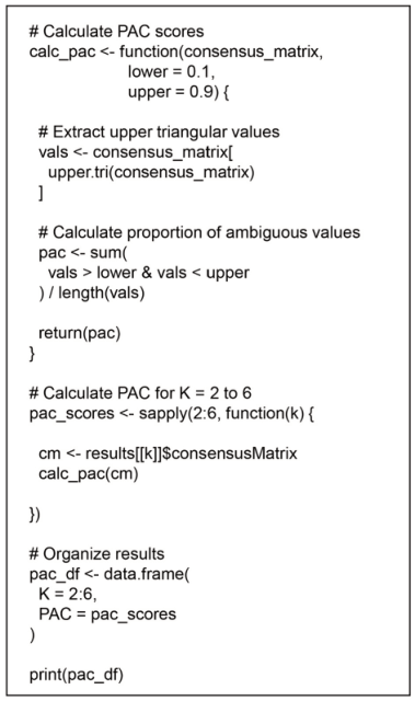
Figure 4. R code for calculating proportion of ambiguous clustering (PAC) scores. PAC was calculated from the upper triangular values of each consensus matrix for K = 2 to K = 6. Consensus values between 0.1 and 0.9 were defined as ambiguous, and the proportion of values within this interval was calculated as the PAC score. K: number of clusters; PAC: proportion of ambiguous clustering.
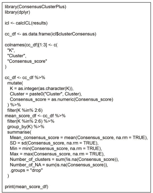
Figure 5. R code for calculating mean cluster consensus scores. Individual cluster consensus scores were summarized for each candidate cluster number from K = 2 to K = 6. The mean cluster consensus score was calculated for each K, together with the standard deviation, minimum, and maximum values. K: number of clusters. for each K, and their mean was used to compare overall within-cluster stability among candidate solutions. Higher cluster consensus scores indicated more consistent grouping of samples within a cluster. For the selected K, individual cluster consensus scores were additionally examined to confirm the stability of each cluster.
The number of samples assigned to each cluster was also recorded for each K to identify solutions containing very small or single-sample clusters. Candidate K values were evaluated using the following sequential procedure. Solutions containing singleton clusters were first excluded, such that a minimum cluster size of two samples was required for a candidate solution to be retained. Among the remaining solutions, within-cluster stability was evaluated using mean cluster consensus. PAC, calculated using an ambiguity interval of 0.1–0.9, and changes in the CDF area were used as complementary measures of clustering ambiguity and incremental stability. Because PAC does not have a universally established absolute cutoff, PAC values were compared across candidate K values rather than interpreted against a fixed threshold. When the stability measures favored different values of K, the more parsimonious solution that maintained high within-cluster consensus without producing very small clusters was retained as the illustrative solution. This approach was used for exploratory cluster selection rather than biological validation of molecular subtypes. Item consensus was additionally examined at the selected K to assess the stability of individual sample assignments. To evaluate sensitivity to feature selection, consensus clustering was repeated using the top 1,000 and 1,500 MAD- ranked genes, and agreement with the original 500-gene solution was assessed using the adjusted Rand index (ARI). In addition, a permutation- based null analysis was performed using 20 permutations by independently permuting expression values across samples within each gene and comparing the resulting PAC values with those obtained from the observed data. The measures used to evaluate candidate values of K are summarized in Table 3, while the PAC values, mean cluster consensus scores, and cluster sizes obtained for each candidate K are presented in Table 4. Common quality-control and troubleshooting considerations for applying the workflow are summarized in Table 5. The main input and output files generated at each step of the workflow are summarized in Table 6.
Table 3. Measures used to evaluate the number of clusters
| Measure | Evaluation | Interpretation |
|---|---|---|
| Consensus matrix | K = 2–6 | Examines within-cluster stability and separation between clusters |
| CDF | K = 2–6 | Shows the distribution of consensus values |
| Delta area | K = 2–6 | Shows the relative change in the area under the CDF curve as K increases |
| PAC | 0–1 | Lower values indicate fewer ambiguous sample pairs |
| Cluster consensus score | 0–1 | Higher values indicate greater within-cluster stability |
| Cluster size | Number of samples | Used to identify very small or single-sample clusters |
| CDF: cumulative distribution function; K: number of clusters; PAC: proportion of ambiguous clustering. | ||
Table 4. Summary of clustering stability metrics and cluster composition across candidate K values
| K | PAC | Mean cluster consensus | Cluster sizes | Singleton cluster |
|---|---|---|---|---|
| 2 | 0.182 | 0.936 | 6, 5 | No |
| 3 | 0.164 | 0.872 | 5, 5, 1 | Yes |
| 4 | 0.182 | 0.728 | 4, 5, 1, 1 | Yes |
| 5 | 0.127 | 0.747 | 2, 5, 2, 1, 1 | Yes |
| 6 | 0.091 | 0.448 | 2, 4, 2, 1, 1, 1 | Yes |
| Lower PAC values indicate fewer ambiguously clustered sample pairs, whereas higher mean cluster consensus values indicate | ||||
| greater within-cluster stability. Cluster sizes represent the number of samples assigned to each cluster. | ||||
| K: number of clusters; PAC: proportion of ambiguous clustering. | ||||
Table 5. Quality-control and troubleshooting guidance for the consensus clustering workflow
| Issue | Possible cause | Recommended action |
|---|---|---|
| NA or infinite values after Z-score transformation | Zero-variance genes | Remove zero-variance genes before Z-score transformation |
| Missing or non-numeric input values | Incomplete or incorrectly formatted input matrix | Resolve missing values and ensure that all expression columns contain numeric values before analysis |
| Unstable consensus matrices | Weak clustering structure or limited sample size | Examine multiple candidate K values and interpret the resulting structure as exploratory |
| Singleton or very small clusters at higher K | Excessive subdivision of samples Consider cluster size when evaluating candidate K values and avoid interpreting very small clusters as robust subgroups | |
| PAC and cluster consensus favor different K values | Stability metrics capture different aspects of clustering | Apply the specified K-selection procedure and interpret the metrics jointly |
| Different results between repeated runs | Random resampling | Set and report a fixed random seed |
| K: number of clusters; NA: not available; PAC: proportion of ambiguous clustering. | ||
Table 6. Summary of input and output files generated during the consensus clustering workflow
| Protocol step | Main input file | Main output file |
|---|---|---|
| MAD calculation | Processed logCPM matrix | Top 500 MAD genes |
| Z-score transformation | Top 500 MAD genes | Z-score expression matrix |
| Consensus clustering | Z-score expression matrix | ConsensusClusterPlus result RDS |
| Evaluation of K | ConsensusClusterPlus result RDS | Consensus matrices, CDF, delta area |
| PAC calculation | Consensus matrices | PAC scores |
| Final cluster assignment | Selected K | Sample cluster assignment file |
| CDF: cumulative distribution function; K: number of clusters; logCPM: log-transformed counts per million; MAD: median | ||
| absolute deviation; PAC: proportion of ambiguous clustering; RDS: R data serialization. | ||
To demonstrate the application of the protocol, the provided processed logCPM expression dataset, consisting of 11 case samples, was used as an example. MAD was calculated for each gene, and the 500 genes with the highest MAD values were selected. Expression values for these genes were converted to gene-wise Z-scores and used as input to ConsensusClusterPlus. Consensus clustering was performed for K = 2 to K = 6 with 1,000 resampling iterations, using 80% of the samples in each iteration. Hierarchical clustering with Pearson correlation was used throughout the analysis.
The consensus matrices showed how the sample grouping changed as the number of clusters increased (Figure 6). At K = 2, the samples were divided into two main groups with relatively clear separation. Additional groups appeared as K increased, resulting in progressively smaller clusters at higher K values. The CDF curves changed with increasing K (Figure 7A). In the delta-area plot, the value at K = 2 represents the total area under the CDF curve and is therefore not directly comparable with the values for K > 2, which represent relative changes in CDF area between successive K values. Among K ≥ 3, the relative change progressively decreased toward higher K values, indicating diminishing changes in the consensus distribution as additional clusters were introduced (Figure 7B).
PAC scores showed a different pattern from the cluster consensus scores. The PAC values for K = 2, 3, 4, 5, and 6 were 0.182, 0.164, 0.182, 0.127, and 0.091, respectively (Figure 7C). The lowest PAC was observed at K = 6, followed by K = 5, whereas K = 2 and K = 4 had the highest values. Based on PAC alone, the higher K solutions therefore contained fewer sample pairs with intermediate consensus values.
In contrast, the mean cluster consensus score was highest at K = 2. The mean scores were 0.936 at K = 2, 0.872 at K = 3, 0.728 at K = 4, 0.747
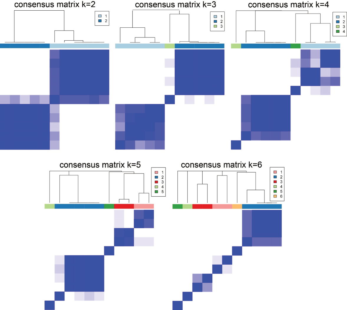
Figure 6. Consensus matrices generated for different numbers of clusters. Consensus matrices are shown for K = 2 to K = 6. Each matrix represents the frequency with which pairs of samples were assigned to the same cluster across 1,000 resampling iterations. Values closer to 1 indicate that two samples were more frequently grouped together, whereas values closer to 0 indicate that they were more frequently assigned to different clusters. K: number of clusters.
at K = 5, and 0.448 at K = 6 (Figure 7D). For the selected K = 2 solution, the individual cluster consensus scores were 0.871 for Cluster 1 and 1.000 for Cluster 2 (Figure 7E). Cluster consensus was thus generally lower when the samples were divided into a larger number of groups, with the largest decrease observed at K = 6. This difference between PAC and cluster consensus shows why the number of clusters should not be chosen from either measure alone.
Cluster composition was also checked when comparing the different solutions, and PAC, mean cluster consensus, and cluster sizes for each candidate K are summarized together in Table 4. Increasing K divided the samples into progressively smaller groups, and the higher K solutions included clusters represented by only a small number of samples. This was considered together with the consensus matrices, CDF and delta area, PAC, and cluster consensus scores when choosing the final cluster number. Although PAC favored a larger K, the K = 2 solution
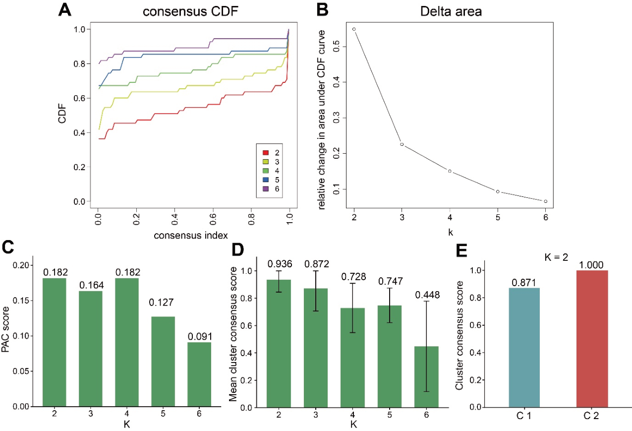
Figure 7. Evaluation of cluster stability across different numbers of clusters. (A) CDF curves of consensus values for K = 2 through K = 6. (B) Delta-area plot. The value at K = 2 represents the total area under the CDF curve, whereas values for K > 2 represent the relative change in CDF area compared with the preceding K. (C) PAC scores for each K (K = 2: 0.182, K = 3: 0.164, K = 4: 0.182, K = 5: 0.127, K = 6: 0.091); lower values indicate fewer ambiguously clustered sample pairs. (D) Mean cluster consensus score at each K (K = 2: 0.936, K = 3: 0.872, K = 4: 0.728, K = 5: 0.747, K = 6: 0.448), with error bars showing the standard deviation across clusters. (E) Cluster consensus scores for each cluster at K = 2 (Cluster 1: 0.871, Cluster 2: 1.000). CDF: cumulative distribution function; K: number of clusters; PAC: proportion of ambiguous clustering.
showed the highest mean cluster consensus score and separated the samples into two main groups without further subdivision into small clusters. K = 2 is presented here as an illustrative example, guided by the combined pattern of these metrics. This is meant only to demonstrate how several stability measures can be read together, not to establish evidence of a genuine molecular subtype structure. Additional analyses were performed to assess the robustness of the illustrative K = 2 solution. Item-consensus scores were generally high for samples assigned to their respective clusters, although one sample showed a comparatively lower item-consensus score of 0.658 (Supplementary Table 2). Sensitivity analyses using the top 500, 1,000, and 1,500 MAD-ranked genes produced identical K = 2 sample assignments, with an ARI of 1.000 for all pairwise comparisons (Supplementary Table 3). The choice of feature-set size should therefore be treated as an analysis parameter and may require sensitivity assessment when the workflow is applied to other datasets. In the permutation-based null analysis, the observed PAC at K = 2 (0.182) was lower than the mean PAC obtained from the null datasets (0.681), whereas the observed and null PAC values became similar at higher K values (Supplementary Table 4). The cluster assignments of the individual samples are shown in Table 7.
Table 7. Example cluster assignments for the illustrative K = 2 solution
| Sample ID | Cluster |
|---|---|
| Case1 | 1 |
| Case2 | 2 |
| Case3 | 1 |
| Case4 | 2 |
| Case5 | 1 |
| Case6 | 1 |
| Case7 | 1 |
| Case8 | 1 |
| Case9 | 2 |
| Case10 | 2 |
| Case11 | 2 |
| K: number of clusters. |
This protocol describes an exploratory consensus clustering workflow for examining potential sample groupings in gene expression data, combining the selection of highly variable genes by MAD, gene-wise Z-score transformation, and clustering with ConsensusClusterPlus. The number of clusters is evaluated using the consensus matrix, CDF, delta area, PAC, cluster consensus score, and cluster size, since these measures provide complementary information about clustering stability and sample grouping.
In the example dataset, PAC favored higher values of K, whereas cluster consensus scores and cluster composition supported a simpler structure with K = 2. This discrepancy illustrates why the number of clusters should be determined by interpreting multiple stability measures together rather than relying on any single metric. Given the small size of the worked example and the absence of independent biological validation, the K = 2 solution should be interpreted only as an exploratory sample grouping rather than as evidence of biologically distinct molecular subtypes.
None.
Conceptualization: Kim J. Data curation: Park D, Ko H. Formal analysis: Park D. Methodology: Park D, Kim J. Software: Park D. Validation: Ko H, Hwang TS. Visualization: Park D. Writing – original draft: Park D. Writing – review & editing: Ko H, Hwang TS, Kim J. Supervision: Kim J. Funding acquisition: Kim J. All authors read and approved the final manuscript.
Jaemin Kim has been the editor-in-chief of Journal of Animal Breeding and Genomics since January 2026. However, she was not involved in the review process of this article. There are no other potential conflicts of interest relevant to this article.
This technical protocol used previously processed gene expression data and involved no new animal experiments or sample collection. Therefore, additional ethical approval was not required.
None.
The following supplementary materials are available on the journal’s website:
• Supplementary Table 1–4
• Supplementary Code: Python, R
During the preparation of this work, the authors used AI to improve the readability and language of the manuscript. After using this tool, the authors reviewed and edited the content as needed and take full responsibility for the content of the publication.
Guinney J, Dienstmann R, Wang X, et al. 2015. The consensus molecular subtypes of colorectal cancer. Nature Medicine 21:1350–1356. https:// doi.org/10.1038/nm.3967
Liu Y, Zhou J, White KP. 2014. RNA-seq differential expression studies: More sequence or more replication? Bioinformatics 30:301–304. https:// doi.org/10.1093/bioinformatics/btt688
Howell DC. 2005. Median absolute deviation. In: Everitt BS, Howell DC, editors. Encyclopedia of statistics in behavioral science. John Wiley & Sons. https://doi.org/10.1002/0470013192.bsa384
Wilkerson MD, Hayes DN. 2010. ConsensusClusterPlus: A class discovery tool with confidence assessments and item tracking. Bioinformatics 26:1572–1573. https://doi.org/10.1093/bioinformatics/btq170
Şenbabaoğlu Y, Michailidis G, Li JZ. 2014. Critical limitations of consensus clustering in class discovery. Scientific Reports 4:6207. https:// doi.org/10.1038/srep06207
Ihaka R, Gentleman R. 1996. R: A language for data analysis and graphics. Journal of Computational and Graphical Statistics 5:299–314. https://doi .org/10.1080/10618600.1996.10474713
Goder A, Filkov V. 2008. Consensus clustering algorithms: Comparison and refinement. In: Munro JI, Wagner D, editors. Proceedings of the Tenth Workshop on Algorithm Engineering and Experiments (ALENEX). SIAM. pp. 109–117. https://doi.org/10.1137/1.9781611972887.11