
Hankyeol Jeong1,2,† , Seongmin Kim1,2,†, Jaemin Kim1,2,*
1Division of Applied Life Science (BK21), Gyeongsang National University, Jinju, Republic of Korea
2Institute of Agriculture and Life Sciences, Gyeongsang National University, Jinju, Republic of Korea
†These authors contributed equally to this work.
Correspondence to Jaemin Kim, E-mail: jmkim85@gnu.ac.kr
Volume 10, Number 2, Pages 51–67, June 2026.
Journal of Animal Breeding and Genomics 2026, 10(2), 51–67. https://doi.org/10.12972/jabng.2026.10.2.3
Received on June 02, 2026, Revised on June 17, 2026, Accepted on June 19, 2026, Published on June 30, 2026.
Copyright © 2026 Korean Society of Animal Breeding and Genetics.
This is an Open Access article distributed under the terms of the Creative Commons Attribution Non-Commercial License (http://creativecommons.org/licenses/by-nc/4.0).

Selective sweep approaches are widely used in livestock population genomics to identify genomic regions affected by positive selection, environmental adaptation, and breed-specific breeding history (Bertolini et al., 2018; Brito et al., 2017). During domestication and breed formation, processes such as genetic drift, reproductive isolation, selective breeding, and environmental pressure shape genomic variation and leave detectable signatures across the genome (Gouveia et al., 2014; Wiener and Wilkinson, 2011). These genomic signatures provide important insights into evolutionary history, adaptation, and economically important traits in domesticated animals.
With the increasing availability of genome-wide SNP genotype data, population genomic approaches have been broadly applied to investigate population structure, genomic inbreeding, and selection signatures in livestock species (Hu et al., 2023; Mdladla et al., 2016; Zhang et al., 2018). Previous studies in goats and other domestic animals have demonstrated that SNP genotype data can effectively identify population differentiation, haplotype structure, and genomic homozygosity patterns associated with selective sweeps and demographic history (Bertolini et al., 2018; Brito et al., 2017; Eydivandi et al., 2021). In particular, approaches such as principal component analysis (PCA), fixation index (FST), cross-population extended haplotype homozygosity (XP-EHH), and runs of homozygosity (ROH) are widely used to characterize genomic patterns associated with adaptation, production traits, and breed formation (Eydivandi et al., 2021; Islam et al., 2019; Waineina et al., 2022).
Goats provide a particularly useful model for demonstrating selective sweep analyses because numerous breeds have been developed for distinct production objectives, including meat, dairy, and fiber (Brito et al., 2017; Zhang et al., 2018). To demonstrate selective sweep analyses among populations with distinct production backgrounds, Boer goats were selected as the target population representing a meat-type breed, whereas Angora and Saanen goats were used as comparison populations representing fiber and dairy production, respectively. Therefore, in this protocol, we describe a practical workflow for detecting selective sweeps using goat SNP genotype data from the publicly available ADAPTmap resource (Colli et al., 2018). Rather than proposing a novel analytical method, this protocol provides a practical and reproducible workflow that integrates widely used population genomic approaches for selective sweep studies. The workflow includes input data preparation and quality control, population structure evaluation, FST-based selective sweep detection, XP-EHH calculation using selscan, and ROH characterization. This protocol aims to provide a reproducible framework for livestock population genomic studies using genome-wide SNP genotype data.
Goat SNP genotype data used in this protocol were obtained from the publicly available ADAPTmap consortium dataset (Colli et al., 2018), which is available through the Dryad public repository (https://datadryad.org/dataset/doi:10.5061/dryad.v8g21pt). The dataset contains goat SNP genotype data generated using the Illumina GoatSNP50 BeadChip platform and provides PLINK binary genotype files for downstream population genomic analyses. Breed metadata information associated with the ADAPTmap dataset was obtained from the supplementary materials of the original publication. Representative goat breeds, including Boer (BOE), Angora (ANG), and Saanen (SAA), were selected for downstream analyses based on breed information provided in the original dataset resource. Boer goats were used as the primary target population for downstream selective sweep analyses, whereas Angora and Saanen populations were used as comparison populations for FST and XP-EHH analyses.
All analyses were performed using autosomal SNP markers located on goat chromosomes 1 to 29. Depending on the analytical objective, multiple genotype data formats were used throughout the workflow, including PLINK binary files and phased genotype files for downstream population genomic analyses. All downstream analyses were performed using consistent chromosome coordinates and marker orders. Population genomic analyses were conducted in a Linux-based computational environment using publicly available software tools. Statistical analyses and visualization were performed in the R environment, whereas Beagle phasing was performed in a Java runtime environment. Table 1 summarizes the major software tools and computational environments used throughout this protocol.
Table 1. Software tools and computational environments used for population genomic analyses
| Category | Software | Version | Purpose |
|---|---|---|---|
| Population genomic analysis | PLINK | v1.90 | SNP filtering, LD pruning, PCA, FST, and ROH analysis |
| Population structure inference | ADMIXTURE | v1.3.0 | Estimation of ancestry proportions |
| Haplotype phasing | Beagle | v5.5 | Generation of phased genotype data |
| Java runtime environment | OpenJDK | v11 | Execution environment for Beagle |
| VCF manipulation | BCFtools | v1.20 | Population-specific VCF extraction |
| Haplotype-based analysis | Selscan | v2.1 | XP-EHH analysis |
| Statistical computing | R | v4.3.1 | Statistical analysis and visualization |
Quality control (QC) procedures were performed to remove low-quality markers and samples before downstream population genetic analyses. QC filtering was performed using PLINK v1.90 on a Linux environment (Chang et al., 2015; Purcell et al., 2007). SNPs with missing or zero physical position values were identified from the .bim file because undefined genomic coordinates can interfere with chromosome-based genomic analyses, window-based summary, and downstream visualization procedures. The Linux command used for this step was as follows:
awk ‘$4 == 0 {print $2}’ \ ADAPTmap_genotypeTOP_20160222_full.bim \ > remove_null-position_list.txt |
The generated exclusion list was saved as a single-column text file containing SNP IDs extracted from the second column of the &.bim* file. This file was subsequently used as the input file for the PLINK &–exclude* option during QC filtering. Each row contained the SNP identifier extracted from the second column of the &.bim* file. Representative goat breeds, including Boer (BOE), Saanen (SAA), and Angora (ANG) populations, were selected from the dataset for downstream analyses based on the breed metadata provided in the original ADAPTmap dataset publication (Colli et al., 2018). Sample information for the selected representative goat breeds was organized as a two-column text file containing Family ID (FID) and Individual ID (IID) for downstream sample retention during QC filtering (Table 2).
Using the SNP exclusion file and the representative goat breed sample list, QC filtering was subsequently performed using the following PLINK command:
plink \ –bfile ADAPTmap_genotypeTOP_20160222_full \ –chr-set 29 \ –chr 1-29 \ –exclude remove_null-position_list.txt \ –geno 0.02 \ –maf 0.01 \ –make-bed \ –mind 0.04 \ –keep keep_breed_list.txt \ –out basic_QC |
The &–chr-set 29* option was used to define the 29 autosomal chromosomes of the goat genome, while the &–chr 1-29* option was used to retain autosomal SNPs for downstream analyses. SNPs listed in the exclusion file were removed using the &–exclude* option, whereas selected representative goat breed samples were retained using the &–keep* option. The &–mind 0.04* option removed samples with individual genotype missing rates greater than 4%, while the &–geno 0.02* option excluded SNPs with genotype missing rates greater than 2% across all samples. In addition, the &–maf 0.01* threshold removed SNPs with minor allele frequencies lower than 0.01. These QC criteria were selected based on the filtering strategy used in the ADAPTmap project and are consistent with thresholds commonly applied in livestock SNP-array population genomic studies (Colli et al., 2018; Liu et al., 2023). After QC filtering, PLINK binary output files (&.bed*, &.bim*, and &.fam*) were generated for downstream analyses. In addition, the &.irem* file contained the list of individuals removed by the &–mind* filtering step. The final QC-filtered dataset comprised 46,463 SNPs and 815 samples and was subsequently used as the common input dataset for downstream LD pruning, PCA, ADMIXTURE, FST, XP-EHH, and ROH analyses described in the downstream workflow (Figure 1).
Table 2. Example structure of the breed retention sample list used for QC filtering
| FID (Family ID) | IID (Individual ID) |
|---|---|
| BOE | AU_BOE0018 |
| SAA | CH_SAA0149 |
| ANG | AR_ANG0154 |
The sample list contains Family ID (FID) and Individual ID (IID) information for individuals retained in the analysis. This file was used with the PLINK –keep option to retain selected goat breeds during quality-control filtering and downstream population genomic analyses.
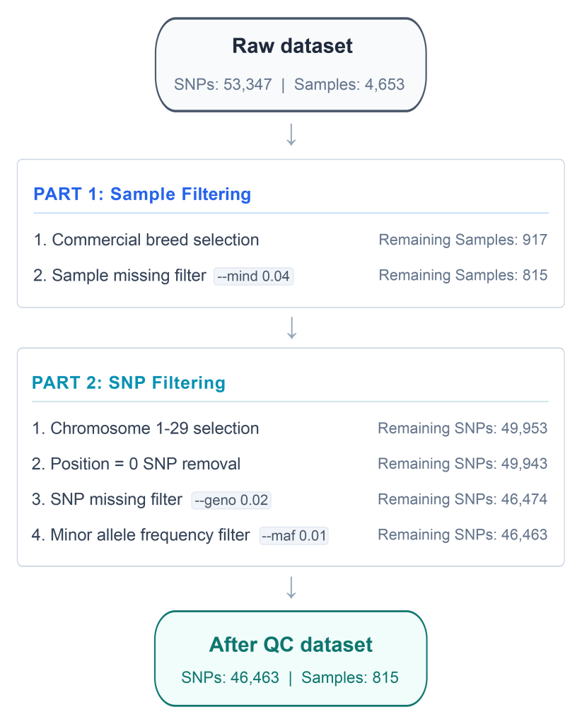
Figure 1. Quality control workflow for goat SNP genotype data
Population structure analysis was performed to evaluate the genetic separation among goat breeds and to determine an appropriate reference population for downstream selective sweep analyses. Before principal component analysis (PCA) and ADMIXTURE analysis, linkage disequilibrium (LD) pruning was performed to reduce the influence of highly correlated SNPs. Because densely linked markers can bias population structure inference by overrepresenting local genomic regions, LD pruning was used to retain a set of approximately independent SNPs for downstream analyses. LD pruning was conducted using PLINK v1.90 with the following command:
|
plink \ –bfile basic_QC \ –chr-set 29 \ –indep-pairwise 50 5 0.2 \ –out LD_pruning |
The &–indep-pairwise 50 5 0.2* option performed LD pruning using a window size of 50 SNPs, a step size of 5 SNPs, and an r昌 threshold of 0.2. These parameters are commonly used in livestock population genomic studies to generate a set of approximately independent markers for population structure inference while retaining sufficient genome-wide variation (Mukhina et al., 2022; Muthusamy et al., 2025; Sun et al., 2024). SNPs showing high pairwise LD were removed to reduce redundancy among neighboring markers and to retain a set of approximately independent SNPs for downstream population structure analyses. PLINK generated two text output files during the LD pruning step: a &.prune.in* file containing SNP markers retained after LD pruning and a &.prune.out* file containing SNP markers excluded because of high pairwise LD. The &.prune.in* file consisted of a single-column text format containing SNP IDs retained as approximately independent markers for downstream analyses. After LD pruning, 17,275 of 46,463 variants were removed, and 29,188 variants were retained. The retained SNP list was subsequently used to construct a new LD-pruned PLINK binary dataset for downstream PCA and ADMIXTURE analyses. This step generated new &.bed*, &.bim*, and &.fam* files containing only the retained approximately independent SNP markers:
|
plink \ –bfile basic_QC \ –chr-set 29 \ –extract LD_pruning.prune.in \ –make-bed \ –out basic_QC_LDpruned |
The LD-pruned dataset was used exclusively for PCA and ADMIXTURE analyses. In contrast, downstream FST, XP-EHH, and ROH analyses were performed using the QC-filtered dataset prior to LD pruning because these analyses require genome-wide marker information and may be influenced by the removal of linked loci.
Principal component analysis (PCA) is a dimension-reduction approach commonly used in population genomics to summarize genetic variation and visualize population-level clustering patterns among individuals (Patterson et al., 2006). To evaluate genetic relationships among goat breeds and identify genetically distinguishable populations for downstream selective sweep analyses, PCA was performed using the LD-pruned dataset generated in the previous step. The following PLINK command was used to calculate principal components from the LD-pruned genotype dataset:
|
plink \ –bfile basic_QC_LDpruned \ –chr-set 29 \ –pca 20 \ –out PCA_LDpruned |
PLINK generated an &.eigenvec* file containing principal component coordinates for each individual and an &.eigenval* file containing the variance explained by each principal component. The &.eigenvec* file was subsequently used for downstream visualization of breed-level clustering patterns among individuals, whereas the &.eigenval* file consisted of a single-column text format containing the eigenvalues corresponding to each principal component (Table 3). The PCA results showed clear genetic differentiation among Boer, Angora, and Saanen goats, with individuals clustering according to breed identity. Boer goats formed a distinct cluster separated from the other breeds along the first principal component, supporting their use as the primary target population for downstream selective sweep analyses (Figure 2).
ADMIXTURE is a model-based clustering method used to estimate ancestry proportions and infer population structure among individuals (Alexander et al., 2009). To assess breed composition and admixture patterns among goat populations, ADMIXTURE analysis was performed using the LD-pruned dataset generated in the previous step. ADMIXTURE was tested for K values ranging from 2 to 4 using the following commands:
|
admixture –cv basic_QC_LDpruned.bed 2 admixture –cv basic_QC_LDpruned.bed 3 admixture –cv basic_QC_LDpruned.bed 4 |
For each K value, ADMIXTURE generated a &.Q* file containing estimated ancestry coefficients for each individual across inferred population clusters and a &.P* file containing estimated allele frequencies for each SNP within each inferred ancestral population (Table 4). The &.Q* file was subsequently used for downstream ADMIXTURE visualization. Cross-validation errors were 0.65642 for K = 2, 0.62772 for K = 3, and 0.61838 for K = 4. Although the lowest CV error was observed at K = 4, the population structure observed at K = 3 showed the clearest correspondence with the known breed composition and PCA clustering patterns. Boer goats showed a relatively homogeneous ancestry component, whereas Angora and Saanen goats displayed distinct breed-level ancestry patterns separated from Boer goats. Consistent with the PCA results, the ADMIXTURE analysis at K = 3 supported clear genetic differentiation among the three major goat breeds included in this study (Figure 3).
It should be noted, however, that the optimal K value does not necessarily correspond to the actual number of breeds, populations, or ancestral groups represented in a dataset (Alexander et al., 2009; Evanno et al., 2005; Puechmaille, 2016). In studies where population structure is unknown or cryptic admixture is expected, examining a broader range of K values may reveal hierarchical population structure, ancestral components, or ongoing admixture events that would otherwise remain undetected (Falush et al., 2003; Lawson et al., 2018). In such contexts, both cross-validation error and biological interpretability should be jointly considered when selecting an appropriate K value. Because the K = 3 structure provided biologically interpretable breed-level differentiation while remaining consistent with PCA-based clustering patterns, K = 3 was considered the most appropriate population structure model for downstream selective sweep analyses.
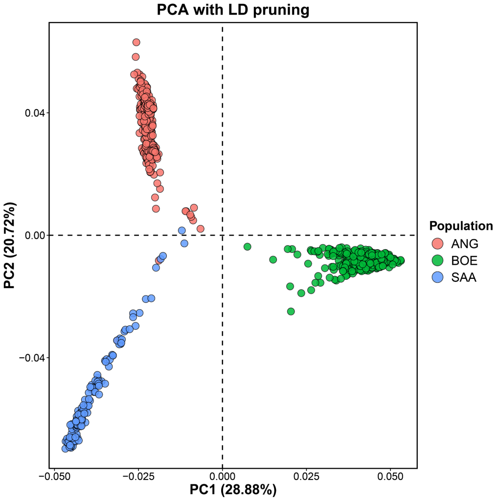
Figure 2. Principal component analysis (PCA) of Boer, Angora, and Saanen goats using LD-pruned SNP markers.
Each point represents an individual goat, colored according to breed. Principal component 1 (PC1) and principal component 2 (PC2) were calculated from the LD-pruned genotype dataset and were used to visualize genetic relationships among populations. The PCA results show clear genetic differentiation among the three goat breeds.
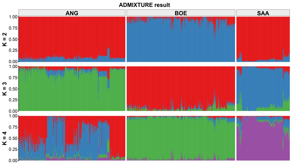
Figure 3. Population ancestry patterns of Boer, Angora, and Saanen goats inferred from ADMIXTURE results at K = 2〝4.
Each vertical bar represents an individual goat, and colored segments indicate the estimated ancestry proportions assigned to each inferred genetic cluster. ADMIXTURE analyses were performed using the LD-pruned genotype dataset with K values ranging from 2 to 4. Individuals are grouped according to breed, allowing visualization of breed composition and population structure among Boer, Angora, and Saanen goats.
Selscan is a haplotype-based program used to detect signatures of selection by estimating extended haplotype homozygosity (EHH). In this protocol, cross-population extended haplotype homozygosity (XP-EHH) analysis is performed to compare haplotype homozygosity patterns between a case population and a control population (Sabeti et al., 2007; Szpiech, 2024). In the practice example presented in this protocol, the Boer population is defined as the case population, whereas Angora and Saanen are used as the control populations. This setup was designed to highlight putative Boer-specific selective sweep signals by contrasting a meat-type commercial breed with breeds selected for different production purposes. Because XP-EHH is a haplotype-based method, phased genotype data without missing genotypes are required.
For XP-EHH analysis, genotype data are converted into phased haplotype format.
|
plink \ –bfile basic_QC \ –recode vcf-iid \ –out basic_QC_recode |
In this protocol, Beagle v5.5 is used to generate phased VCF files required for XP-EHH analysis (Browning et al., 2021). Before phasing, the whole-genome VCF file is split by chromosome, and chromosome-specific VCF files are generated for goat autosomes, chromosomes 1 to 29. Each chromosome-specific VCF file is then used as input for Beagle to produce phased VCF files for downstream XP-EHH analysis.
|
java -Xmx50g -jar beagle.27Feb25.75f.jar \ gt=basic_QC_chr${CHR}.vcf.gz \ out=basic_QC_chr${CHR}.beagle_phased basic_QC_chr${CHR}.beagle_phased.vcf.gz basic_QC_chr${CHR}.beagle_phased.log bcftools view \ -S Boer.txt \ -Oz \ -o Boer.chr${CHR}.beagle_phased.vcf.gz \ basic_QC_chr${CHR}.beagle_phased.vcf.gz bcftools view \ -S Angora_Saanen.txt \ -Oz \ -o Angora_Saanen.chr${CHR}.beagle_phased.vcf.gz \ basic_QC_chr${CHR}.beagle_phased.vcf.gz |
After Beagle phasing, chromosome-specific phased VCF files are separated into case and control population-specific VCF files. This step is performed using the -S option of bcftools view (Danecek et al., 2021), which requires a text file containing the sample IDs to be retained in each population. The resulting case phased VCF file is used as the –vcf input for selscan, whereas the control phased VCF file is used as the –vcf-ref input. Because the direction of the XP-EHH score depends on the input order of –vcf and –vcf-ref, the case-control input direction should be kept consistent throughout the analysis. For XP-EHH analysis, chromosome-specific map files are generated in the input format required by selscan. The selscan map file consists of four columns: chromosome, SNP ID, genetic position, and physical position. PLINK .map files are first generated from chromosome-specific VCF files using the –recode option (Chang et al., 2015; Purcell et al., 2007). If species-specific genetic map information is not available, the physical position of each SNP can be divided by 1,000,000 and used as a pseudo-genetic position. The final map file is prepared without a header and must contain the same SNP marker set and marker order as the case and control phased VCF files used for XP-EHH analysis (Table 5).
|
plink \ –vcf basic_QC_chr${CHR}.beagle_phased.vcf.gz \ –recode \ –allow-extra-chr \ –allow-no-sex \ –cow \ –out Tech_chr${CHR} awk -v chr=${CHR} ‘BEGIN{OFS=”\t”} {print chr, $2, $4/1000000, $4}’ \ Tech_chr${CHR}.map > selscan_chr${CHR}.map |
XP-EHH analysis is performed independently for each chromosome using the case phased VCF file, the control phased VCF file, and the corresponding chromosome-specific map file. After running selscan, raw XP-EHH output files and log files are generated for each chromosome. Because raw XP-EHH scores are not standardized, genome-wide normalization is performed using the norm program before downstream analysis.
After normalization, positive normalized XP-EHH scores indicate increased haplotype homozygosity in the population specified by –vcf, which corresponds to the case population in this protocol. In contrast, negative normalized XP-EHH scores indicate increased haplotype homozygosity in the population specified by –vcf-ref, which corresponds to the control population. Therefore, the direction of the normalized XP-EHH score should be interpreted according to the input order of the case and control populations.
|
selscan \ –xpehh \ –vcf Boer.chr${CHR}.beagle_phased.vcf \ –vcf-ref Angora_Saanen.chr${CHR}.beagle_phased.vcf \ –map chr${CHR}.map \ –out xpehh.chr${CHR}.Boer_vs_AngoraSaanen |
Normalized XP-EHH scores can be visualized at either the SNP level or the window level. SNP-level visualization uses the normalized XP-EHH score of each SNP directly and is typically presented as a Manhattan plot. This approach is useful for examining detailed SNP-level signals across the genome. Window-level visualization summarizes XP-EHH scores at the genomic region level. In this protocol, each chromosome is divided into non-overlapping genomic windows, and the maximum normalized XP-EHH score within each window is used as the representative value. This approach reduces SNP-level variation into regional patterns and can be useful for identifying candidate selection regions. Therefore, SNP-level and window-level plots can be used as complementary visualization strategies depending on the analysis objective, marker density, and downstream criteria used to define candidate selection regions (Figure 4).
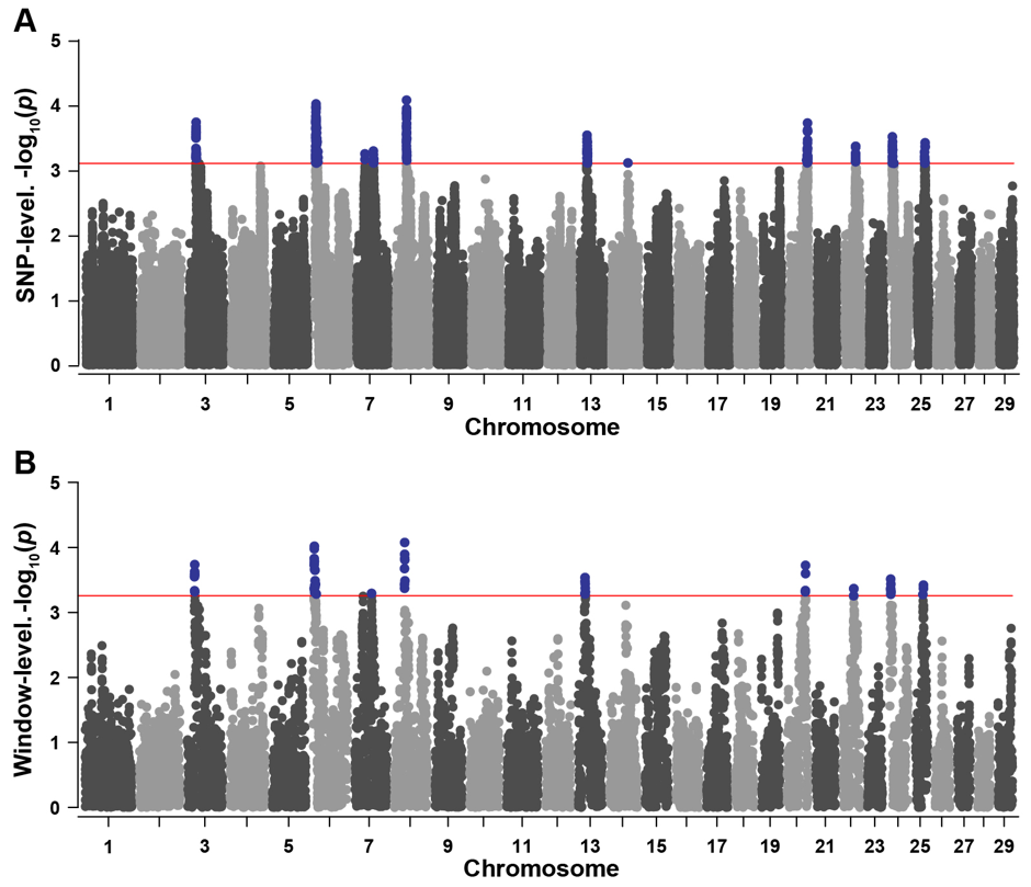
Figure 4. SNP-level and window-level XP-EHH scores Manhattan plots between Boer goats and the comparison populations.
(A) SNP-level XP-EHH Manhattan plot showing normalized XP-EHH scores for individual SNPs across the genome. (B) Window-level XP-EHH Manhattan plot showing the maximum normalized XP-EHH score within each non-overlapping genomic window. The horizontal red line indicates the significance threshold used to identify candidate selective sweep signals, and highlighted points represent genomic regions exceeding this threshold.
Fixation index (FST) is a population differentiation statistic widely used to quantify allele frequency divergence between populations (Weir and Cockerham, 1984). Because selective sweeps can increase genetic differentiation at specific genomic regions, FST-based approaches are used to identify candidate regions under selection in population genomic studies. In this protocol, FST analysis was performed to identify genomic regions showing increased genetic differentiation between Boer goats and the comparison populations. For FST analysis, Boer goats were defined as the target population, whereas Angora and Saanen goats were combined and used as the comparison population. Population-specific sample list files were first generated from the PLINK &.fam* file using Linux commands to retain individuals belonging to the target and comparison populations during downstream FST analysis. Separate sample list files were prepared for the Boer target population (&BOE*) and the combined comparison population (&REF*), which consisted of Angora and Saanen individuals. Each sample list file followed the same two-column PLINK sample selection format described previously in Table 2 and contained Family ID (FID) and Individual ID (IID) information for the retained individuals. A separate population cluster file was then prepared to define the target and comparison population assignments required for PLINK-based FST calculation. The cluster file consisted of three columns corresponding to FID, IID, and population label, where each sample was assigned either to the Boer target population (&BOE*) or to the combined comparison population (&REF*)(Table 6). This cluster file was subsequently used with the &–within* option to specify population membership information during FST estimation. SNP-level FST values were calculated using PLINK v1.90 with the following command:
plink \ –bfile basic_QC \ –chr-set 29 \ –keep BOE_REF_sample_list.txt \ –within BOE_REF_cluster.txt \ –fst \ –out FST_BOE_vs_REF |
The &.fst* output file generated by PLINK contained chromosome number, SNP identifier, physical position, sample count, and SNP-level FST estimates for each marker. These SNP-level FST values were subsequently used for genome-wide visualization and downstream window-level summarization. Because selective sweeps often produce localized increases in population differentiation, SNP-level FST estimates can be used to identify candidate genomic regions showing elevated divergence between the target and comparison populations. Although SNP-level FST signals are useful for examining marker-level differentiation patterns across the genome, individual SNP signals can be influenced by stochastic variation, local marker density, or isolated high-FST loci. Therefore, window-level summarization can additionally be applied to reduce SNP-level noise and to identify broader genomic regions showing consistent differentiation patterns associated with selective sweeps. For regional summarization, the genome was divided into non-overlapping 200-kb windows, and the maximum FST value within each window was used as the representative statistic for downstream visualization and candidate region screening. This approach enables localized differentiation peaks to be summarized as regional selective sweep signals while preserving highly differentiated loci within each genomic window. Window-level FST values were generated using the following R workflow:
library(dplyr) fst <- read.table(“FST_BOE_vs_REF.fst”, header = TRUE, sep = “\t”) fst <- fst %>% filter(!is.na(FST)) window_size <- 200000 fst_window <- fst %>% mutate( WINDOW_START = floor(POS / window_size) * window_size, WINDOW_END = WINDOW_START + window_size ) %>% |
group_by(CHR, WINDOW_START, WINDOW_END) %>% summarise( max_FST = max(FST, na.rm = TRUE), mean_FST = mean(FST, na.rm = TRUE), n_SNP = n(), .groups = “drop” ) write.table(fst_window, “FST_BOE_vs_REF_200kb_window.txt”, sep = “\t”, quote = FALSE, row.names = FALSE) |
Candidate selective sweep regions can subsequently be identified by selecting genomic windows exceeding a user-defined empirical threshold determined according to the analytical objective, population structure, marker density, and the overall distribution of window-level FST values. Depending on the analysis objective, SNP-level and window-level Manhattan plots can be interpreted either independently or together as complementary visualization strategies. SNP-level plots provide marker-resolution differentiation patterns, whereas window-level plots facilitate regional interpretation of broader selective sweep signals across the genome. In this protocol, both visualization strategies were used to examine genome-wide differentiation patterns and candidate selective sweep regions between Boer goats and the comparison populations (Figure 5).
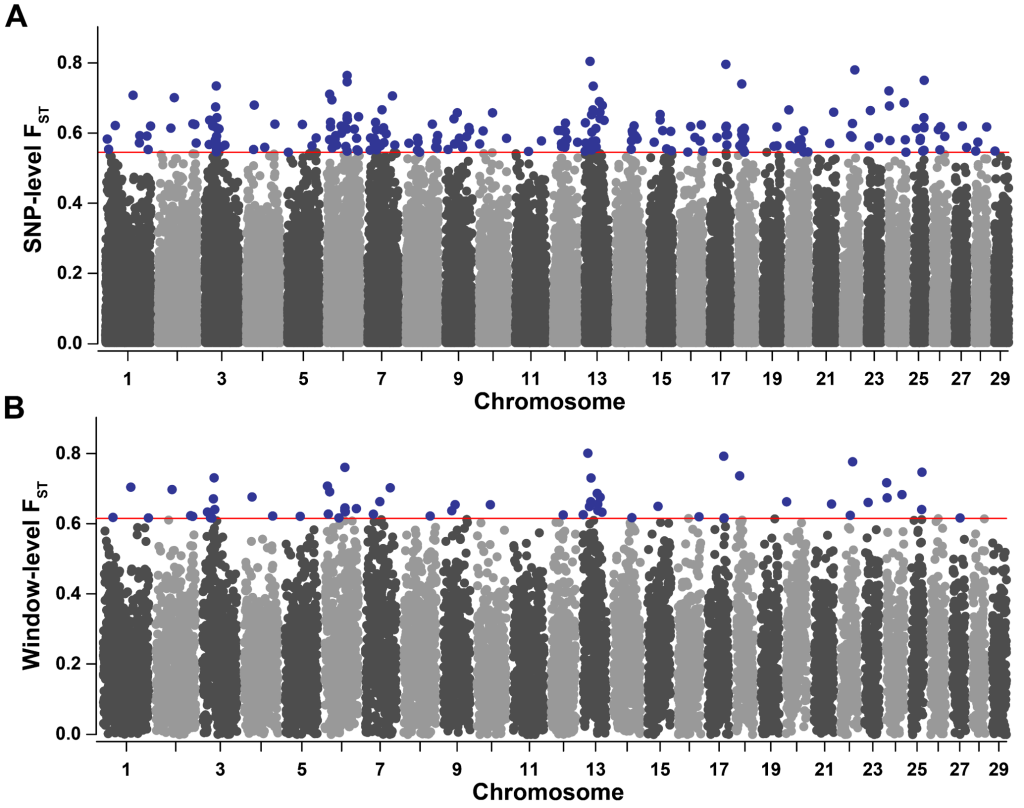
Figure 5. SNP-level and window-level FST Manhattan plots between Boer goats and the comparison populations.
(A) SNP-level FST Manhattan plot showing marker-level genetic differentiation across the genome. (B) Window-level FST Manhattan plot showing the maximum FST value within each non-overlapping genomic window. The horizontal red line indicates the threshold used to identify candidate selective sweep regions, and highlighted points represent genomic regions exceeding this threshold.
PLINK v1.9 is a command-line genotype analysis program used for large-scale genotype data filtering, format conversion, and population genetic analyses. In this protocol, individual ROH segments are detected using the –homozyg option in PLINK v1.9. The –homozyg option detects ROH segments based on the PLINK 1.07 scanning algorithm and allows users to specify detailed parameters, including the minimum number of SNPs, minimum segment length, maximum gap between SNPs, scanning window size, and the number of heterozygous and missing genotype calls allowed within each scanning window (Table 7) (Meyermans et al., 2020). In the practice example, ROH detection was performed using –homozyg-snp 20, –homozyg-kb 1000, –homozyg-gap 500, –homozyg-window-snp 20, –homozyg-window-het 0, and –homozyg-window-missing 2, while other –homozyg parameters were left at the default PLINK settings. These settings were selected based on commonly used SNP-array-based ROH criteria (Lencz et al., 2007) and livestock ROH studies, including goat populations (Cortellari et al., 2021). The minimum length and SNP number thresholds were applied to reduce false-positive ROH calls, the maximum gap threshold was used to avoid merging distant homozygous regions, and the window-based heterozygous and missing genotype criteria were set to maintain stringent but practical ROH detection.
ROH results were summarized at the individual and breed levels using the .hom file generated by the –homozyg option in PLINK. In this protocol, the number of ROH segments detected in each individual was defined as NROH, and the summed length of all ROH segments within each individual was calculated as SROH. SROH was converted and expressed in megabases (Mb). NROH represents the number of ROH segments per individual, whereas SROH represents the total genomic length covered by ROH segments. Individual-level NROH and SROH values were visualized together to assess ROH burden patterns across populations. This approach allows comparison of whether ROH burden is mainly characterized by a larger number of ROH segments, a greater cumulative ROH length, or both. ROH segments were further classified into four length classes: 1〝2 Mb, 2〝4 Mb, 4〝8 Mb, and ‾8 Mb. In general, shorter ROH segments may reflect older shared ancestry, historical bottlenecks, or long-term reductions in effective population size, whereas longer ROH segments are more likely to indicate recent inbreeding or recent population bottlenecks.
NROH and SROH were summarized across ROH length classes to evaluate the length composition of ROH burden. This analysis helps determine whether the overall ROH burden is mainly driven by numerous short ROH segments or by the cumulative contribution of longer ROH segments. Because ROH detection can be affected by SNP density, marker distribution, missing genotypes, quality control criteria, and PLINK –homozyg parameter settings, population-level comparisons should be interpreted based on results generated using the same filtering criteria and ROH detection parameters (Figure 6).
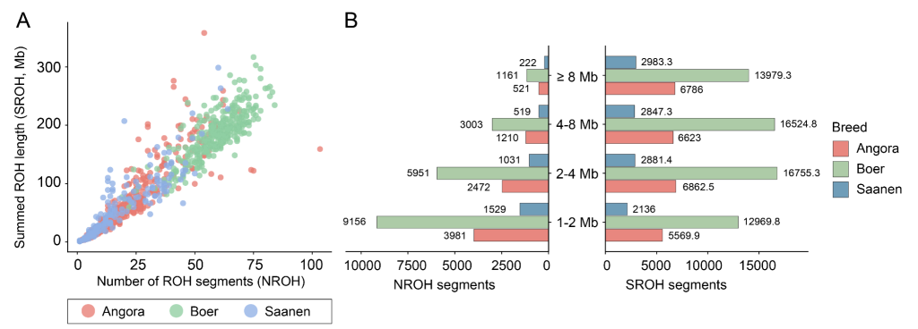
Figure 6. ROH burden across individuals and length classes.
(A) Relationship between the number of ROH segments (NROH) and the summed ROH length (SROH) for individual goats. Each point represents an individual, and colors indicate breed assignment. (B) Breed-level distributions of ROH burden across four ROH length classes (1〝2 Mb, 2〝4 Mb, 4〝8 Mb, and ‾8 Mb), summarized using both the number of ROH segments (NROH) and the summed ROH length (SROH).
This protocol describes procedures for selective sweep studies using publicly available goat SNP genotype data. Genotype quality control, population structure characterization, fixation index (FST), cross-population extended haplotype homozygosity (XP-EHH), and runs of homozygosity (ROH) were presented using representative goat breeds. To facilitate practical implementation, the input and output file formats generated at each analytical step are summarized in Table 8. The workflow described in this study may be useful for livestock population genomic studies using genome-wide SNP genotype datasets.
This research was supported by Basic Science Research Program through the National Research Foundation of Korea (NRF) funded by the Ministry of Education (No.\RS-2025-25431741)
1. Alexander DH, Novembre J, Lange K. 2009. Fast model-based estimation of ancestry in unrelated individuals. Genome research 19(9):1655.
[DOI][PubMed][PMC]
2. Bertolini F, Cardoso TF, Marras G, Nicolazzi EL, Rothschild MF, Amills M, Consortium A. 2018. Genome-wide patterns of homozygosity provide clues about the population history and adaptation of goats. Genetics Selection Evolution 50(1):59.
[DOI][PubMed][PMC]
3. Bertolini F, Servin B, Talenti A, Rochat E, Kim ES, Oget C, Palhière I, Crisà A, Catillo G, Steri R. 2018. Signatures of selection and environmental adaptation across the goat genome post-domestication. Genetics Selection Evolution 50(1):57.
[DOI][PubMed][PMC]
4. Brito LF, Kijas JW, Ventura RV, Sargolzaei M, Porto-Neto LR, Cánovas A, Feng Z, Jafarikia M, Schenkel FS. 2017. Genetic diversity and signatures of selection in various goat breeds revealed by genome-wide SNP markers. BMC genomics 18(1):229.
[DOI][PubMed][PMC]
5. Browning BL, Tian X, Zhou Y, Browning SR. 2021. Fast two-stage phasing of large-scale sequence data. The American journal of human genetics 108(10):1880-1890.
[DOI][PubMed][PMC]
6. Chang CC, Chow CC, Tellier LC, Vattikuti S, Purcell SM, Lee JJ. 2015. Second-generation PLINK: rising to the challenge of larger and richer datasets. GigaScience 4(1):s13742-015-0047-8.
[DOI][PubMed][PMC]
7. Colli L, Milanesi M, Talenti A, Bertolini F, Chen M, Crisà A, Daly KG, Del Corvo M, Guldbrandtsen B, Lenstra JA. 2018. Genome-wide SNP profiling of worldwide goat populations reveals strong partitioning of diversity and highlights post-domestication migration routes. Genetics Selection Evolution 50(1):58.
[DOI][PubMed][PMC]
8. Cortellari M, Bionda A, Negro A, Frattini S, Mastrangelo S, Somenzi E, Lasagna E, Sarti FM, Ciani E, Ciampolini R. 2021. Runs of homozygosity in the Italian goat breeds: impact of management practices in low-input systems. Genetics Selection Evolution 53(1):92.
[DOI][PubMed][PMC]
9. Danecek P, Bonfield JK, Liddle J, Marshall J, Ohan V, Pollard MO, Whitwham A, Keane T, McCarthy SA, Davies RM et al. 2021. Twelve years of SAMtools and BCFtools. GigaScience 10(2).
[DOI][PubMed][PMC]
10. Evanno G, Regnaut S, Goudet J. 2005. Detecting the number of clusters of individuals using the software STRUCTURE: a simulation study. Molecular ecology 14(8):2611-2620.
[DOI][PubMed]
11. Eydivandi S, Roudbar MA, Karimi MO, Sahana G. 2021. Genomic scans for selective sweeps through haplotype homozygosity and allelic fixation in 14 indigenous sheep breeds from Middle East and South Asia. Scientific Reports 11(1):2834.
[DOI][PubMed][PMC]
12. Falush D, Stephens M, Pritchard JK. 2003. Inference of population structure using multilocus genotype data: linked loci and correlated allele frequencies. Genetics 164(4):1567-1587.
[DOI][PubMed][PMC]
13. Gouveia JJdS, Silva MVGBd, Paiva SR, Oliveira SMPd. 2014. Identification of selection signatures in livestock species. Genetics and molecular biology 37(2):330-342.
[DOI][PubMed][PMC]
14. Hu M, Jiang H, Lai W, Shi L, Yi W, Sun H, Chen C, Yuan B, Yan S, Zhang J. 2023. Assessing genomic diversity and signatures of selection in Chinese red steppe cattle using high-density SNP Array. Animals 13(10):1717.
[DOI][PubMed][PMC]
15. Islam R, Li Y, Liu X, Berihulay H, Abied A, Gebreselassie G, Ma Q, Ma Y. 2019. Genome-wide runs of homozygosity, effective population size, and detection of positive selection signatures in six Chinese goat breeds. Genes 10(11):938.
[DOI][PubMed][PMC]
16. Lawson DJ, Van Dorp L, Falush D. 2018. A tutorial on how not to over-interpret STRUCTURE and ADMIXTURE bar plots. Nature Communications 9(1):3258.
[DOI][PubMed][PMC]
17. Lencz T, Lambert C, DeRosse P, Burdick KE, Morgan TV, Kane JM, Kucherlapati R, Malhotra AK. 2007. Runs of homozygosity reveal highly penetrant recessive loci in schizophrenia. Proceedings of the National Academy of Sciences 104(50):19942-19947.
[DOI][PubMed][PMC]
18. Liu Z, Fu S, He X, Liu X, Shi C, Dai L, Wang B, Chai Y, Liu Y, Zhang W. 2023. Estimates of genomic heritability and the marker-derived gene for re (production) traits in Xinggao sheep. Genes 14(3):579.
[DOI][PubMed][PMC]
19. Mdladla K, Dzomba E, Huson H, Muchadeyi F. 2016. Population genomic structure and linkage disequilibrium analysis of South African goat breeds using genome‐wide SNP data. Animal genetics 47(4):471-482.
[DOI][PubMed]
20. Meyermans R, Gorssen W, Buys N, Janssens S. 2020. How to study runs of homozygosity using PLINK? A guide for analyzing medium density SNP data in livestock and pet species. BMC genomics 21(1).
[DOI][PubMed][PMC]
21. Mukhina V, Svishcheva G, Voronkova V, Stolpovsky Y, Piskunov A. 2022. Genetic diversity, population structure and phylogeny of indigenous goats of Mongolia revealed by SNP genotyping. Animals 12(3):221.
[DOI][PubMed][PMC]
22. Muthusamy M, Akinsola OM, Pal P, Ramasamy C, Ramasamy S, Musa AA, Thiruvenkadan AK. 2025. Comparative genomic insights into adaptation, selection signatures, and population dynamics in indigenous Indian sheep and foreign breeds. Frontiers in Genetics 16:1621960.
[DOI][PubMed][PMC]
23. Patterson N, Price AL, Reich D. 2006. Population structure and eigenanalysis. PLoS genetics 2(12):e190.
[DOI][PubMed][PMC]
24. Puechmaille SJ. 2016. The program structure does not reliably recover the correct population structure when sampling is uneven: subsampling and new estimators alleviate the problem. Molecular ecology resources 16(3):608-627.
[DOI][PubMed]
25. Purcell S, Neale B, Todd-Brown K, Thomas L, Ferreira MA, Bender D, Maller J, Sklar P, De Bakker PI, Daly MJ. 2007. PLINK: a tool set for whole-genome association and population-based linkage analyses. The American journal of human genetics 81(3):559-575.
[DOI][PubMed][PMC]
26. Sabeti PC, Varilly P, Fry B, Lohmueller J, Hostetter E, Cotsapas C, Xie X, Byrne EH, McCarroll SA, Gaudet R et al. 2007. Genome-wide detection and characterization of positive selection in human populations. Nature 449(7164):913-8.
[DOI][PubMed][PMC]
27. Sun X, Guo J, Li R, Zhang H, Zhang Y, Liu GE, Emu Q, Zhang H. 2024. Whole-genome resequencing reveals genetic diversity and wool trait-related genes in liangshan semi-fine-wool sheep. Animals 14(3):444.
[DOI][PubMed][PMC]
28. Szpiech ZA. 2024. selscan 2.0: scanning for sweeps in unphased data. Bioinformatics 40(1).
[DOI][PubMed][PMC]
29. Waineina RW, Okeno TO, Ilatsia ED, Ngeno K. 2022. Selection signature analyses revealed genes associated with adaptation, production, and reproduction in selected goat breeds in Kenya. Frontiers in Genetics 13:858923.
[DOI][PubMed][PMC]
30. Weir BS, Cockerham CC. 1984. Estimating F-statistics for the analysis of population structure. evolution:1358-1370.
[DOI][PubMed][PMC]
31. Wiener P, Wilkinson S. 2011. Deciphering the genetic basis of animal domestication. Proceedings of the Royal Society B: Biological Sciences 278(1722):3161-3170.
[DOI][PubMed][PMC]
32. Zhang B, Chang L, Lan X, Asif N, Guan F, Fu D, Li B, Yan C, Zhang H, Zhang X. 2018. Genome-wide definition of selective sweeps reveals molecular evidence of trait-driven domestication among elite goat (Capra species) breeds for the production of dairy, cashmere, and meat. GigaScience 7(12):giy105.
[DOI][PubMed][PMC]